C is for clipping
Previously in our A to Z series we covered seismic amplitude and bit depth. Bit depth determines how smooth the amplitude histogram is. Clipping describes what happens when this histogram is truncated. It is often done deliberately to allow more precision for the majority of samples (in the middle of the histogram), but at the cost of no precision at all for extreme values (at the ends of the histogram). One reason to do this, for example, might be when loading 16- or 32-bit data into a software application that can only use 8-bit data (e.g. most volume interpretation software).
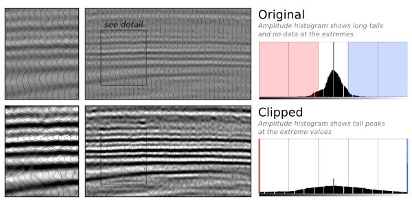
Let's look at an example. Suppose we start with a smooth, unclipped dataset represented by 2-byte integers, as in the top upper image in the figure below. Its histogram, to the right, is a close approximation to a bell curve, with no samples, or very few, at the extreme values. In a 16-bit volume, remember, these extreme values are -32 767 and +32 768. In other words, the data fit entirely within the range allowed by the bit-depth.
 Data from F3 dataset, offshore Netherlands, from the OpendTect Open Seismic Repository.
Now imagine we have to represent this data with 1-byte samples, or a bit-depth of 8. In the lower part of the figure, you see the data after this transformation with its histogram is to the right. Look at the extreme ends of the histogram: there is a big spike of samples there. All of the samples in the tails of the unclipped histogram (shown in red and blue) have been crammed into those two values: -127 and +128. For example, any sample with an amplitude of +10 000 or more in the unclipped data, now has a value of +128. Likewise, amplitudes of –10 000 or less are all now represented by a single amplitude: –127. Any nuance or subtlety in the data in those higher-magnitude samples has gone forever.
Notice the upside though: the contrast of the unclipped data has been boosted, and we might feel like we can see more detail and discriminate more features in this display. Paradoxically, there is less precision, but perhaps it's easier to interpret.
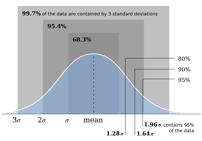
 How much data did we affect? We remember to pull out our basic cheatsheet and look at the normal distribution, below. If we clip the data at about two standard deviations from the mean, then we are only affecting 4.2% of the samples in the data. This might include lots of samples of little quantitative interest (the sea-floor, for example), but is also likely to include samples you do care about: bright amplitudes in or near the zone of interest. For this reason, while clipping might not affect how you interpret the structural framework of your earth model, you need to be aware of it in any quantitative work.
Have you ever been tripped up by clipped seismic data? Do you think it should be avoided at all costs, or maybe you have a tip for avoiding severe clipping? Leave a comment!