Unsolved problems in applied geoscience

I like unsolved problems. I first wrote about them way back in late 2010 — Unsolved problems was the eleventh post on this blog. I touched on the theme again in 2013, before and after the first 'unsession' at the GeoConvention, which itself was dedicated to finding the most pressing questions in exploration geoscience. As we turn towards the unsession at AAPG in Salt Lake City in May, I find myself thinking again about unsolved problems. Specifically, what are they? How can we find them? And what can we do to make them easier to solve?

It turns out lots of people have asked these questions before.

I've compiled a list of various attempts by geoscientists to list he big questions in the field. The only one I was previous aware of was Milo Backus's challenges in applied seismic geophysics, laid out in his president's column in GEOPHYSICS in 1980 and highlighted later by Larry Lines as part of the SEG's 75th anniversary. Here are some notable attempts:

• John William Dawson, 1883 — Nova Scotia's most famous geologist listed unsolved problems in geology in his presidential address to the American Association for the Advancement of Science. They included the Cambrian Explosion, and the origin of the Antarctic icecap. 
• Leason Heberling Adams, 1947 — One of the first experimental rock physicists, Adams made the first list I can find in geophysics, which was less than 30 years old at the time. He included the origin of the geomagnetic field, and the temperature of the earth's interior.
• Milo Backus, 1980 — The list included direct hydrocarbon detection, seismic imaging, attenuation, and anisotropy.  
• Mary Lou Zoback, 2000 — As her presidential address to the GSA, Zoback kept things quite high-level, asking questions about finding signal indynamic systems, defining mass flux and energy balance, identifying feedback loops, and communicating uncertainty and risk. This last one pops up in almost every list since.
• Calgary's geoscience community, 2013 — The 2013 unsession unearthed a list of questions from about 50 geoscientists. They included: open data, improving seismic resolution, dealing with error and uncertainty, and global water management.
• Daniel Garcia-Castellanos, 2014 — The Retos Terrícolas blog listed 49 problems in 7 categories, ranging from the early solar system to the earth's interior, plate tectonics, oceans, and climate. The list is still maintained by Daniel and pops up occasionally on other blogs and on Wikipedia.

The list continues — you can see them all in this presentation I made for a talk (online) at the Bureau of Economic Geology last week (thank you to Sergey Fomel for hosting me!). During the talk, I took the opportunity to ask those present what their unsolved problems are, especially the ones in their own fields. Here are a few of what we got (the rest are in the preso):

What are your unsolved problems in applied geoscience? Share them in the comments!

---

If you have about 50 minutes to spare, you can watch the talk here, courtesy of BEG's streaming service.

Click here to watch the talk >>>

What is scientific computing?

I started my career in sequence stratigraphy, so I know a futile discussion about semantics when I see one. But humour me for a second.

As you may know, we offer a multi-day course on 'geocomputing'. Somebody just asked me: what is this mysterious, made-up-sounding discipline? Swiftly followed by: can you really teach people how to do computational geoscience in a few days? And then: can YOU really teach people anything??

Good questions

You can come at the same kind of question from different angles. For example, sometimes professional programmers get jumpy about programming courses and the whole "learn to code" movement. I think the objection is that programming is a profession, like other kinds of engineering, and no-one would dream of offering a 3-day course on, say, dentistry for beginners.

These concerns are valid, sort of.

1. No, you can't learn to be a computational scientist in 3 days. But you can make a start. A really good one at that.
2. And no, we're not programmers. But we're scientists who get things done with code. And we're here to help.
3. And definitely no, we're not trying to teach people to be software engineers. We want to see more computational geoscientists, which is a different thing entirely.

So what's geocomputing then?

Words seem inadequate for nuanced discussion. Let's instead use the language of ternary diagrams. Here's how I think 'scientific computing' stacks up against 'computer science' and 'software engineering'...

View fullsize

If you think these are confusing, just be glad I didn't go for tetrahedrons.

These are silly, of course. We could argue about them for hours I'm sure. Where would IT fit? ("It's all about the business" or something like that.) Where does Agile fit? (I've caricatured our journey, or tried to.) Where do you fit? 

The Surmont Supermerge

In my recent Abstract horror post, I mentioned an interesting paper in passing, Durkin et al. (2017):

Paul R. Durkin, Ron L. Boyd, Stephen M. Hubbard, Albert W. Shultz, Michael D. Blum (2017). Three-Dimensional Reconstruction of Meander-Belt Evolution, Cretaceous Mcmurray Formation, Alberta Foreland Basin, Canada. Journal of Sedimentary Research 87 (10), p 1075–1099. doi: 10.2110/jsr.2017.59

I wanted to write about it, or rather about its dataset, because I spent about 3 years of my life working on the USD 75 million seismic volume featured in the paper. Not just on interpreting it, but also on acquiring and processing the data.

Let's start by feasting our eyes on a horizon slice, plus interpretation, of the Surmont 'Supermerge' 3D seismic volume:

Figure 1 from Durkin et al (2017), showing a stratal slice from 10 ms below the top of the McMurray Formation (left), and its interpretation (right). © 2017, SEPM (Society for Sedimentary Geology) and licensed CC-BY.

A decade ago, I was 'geophysics advisor' on Surmont, which is jointly operated by ConocoPhillips Canada, where I worked, and Total E&P Canada. My line manager was a Total employee; his managers were ex-Gulf Canada. It was a fantastic, high-functioning team, and working on this project had a profound effect on me as a geoscientist. 

The Surmont bitumen field

The dataset covers most of the Surmont lease, in the giant Athabasca Oil Sands play of northern Alberta, Canada. The Surmont field alone contains something like 25 billions barrels of bitumen in place. It's ridiculously massive — you'd be delighted to find 300 million bbl offshore. Given that it's expensive and carbon-intensive to produce bitumen with today's methods — steam-assisted gravity drainage (SAGD, "sag-dee") in Surmont's case — it's understandable that there's a great deal of debate about producing the oil sands. One factoid: you have to burn about 1 Mscf or 30 m³ of natural gas, costing about USD 10–15, to make enough steam to produce 1 bbl of bitumen.

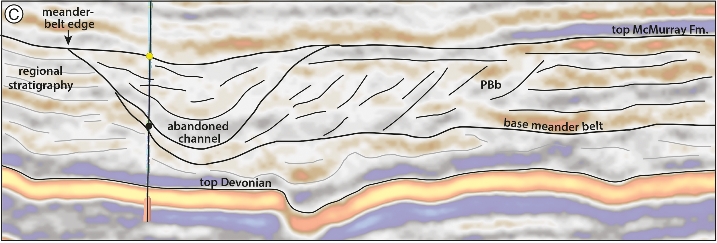
Detail from Figure 12 from Durkin et al (2017), showing a seismic section through the McMurray Formation. Most of the abandoned channels are filled with mudstone (really a siltstone). The dipping heterolithic strata of the point bars, so obvious in horizon slices, are quite subtle in section. © 2017, SEPM (Society for Sedimentary Geology) and licensed CC-BY.

The field is a geoscience wonderland. Apart from the 600 km² of beautiful 3D seismic, there are now about 1500 wells, most of which are on the 3D. In places there are more than 20 wells per section (1 sq mile, 2.6 km², 640 acres). Most of the wells have a full suite of logs, including FMI in 2/3 wells and shear sonic as well in many cases, and about 550 wells now have core through the entire reservoir interval — about 65–75 m across most of Surmont. Let that sink in for a minute.

What's so awesome about the seismic?

OK, I'm a bit biased, because I planned the acquisition of several pieces of this survey. There are some challenges to collecting great data at Surmont. The reservoir is only about 500 m below the surface. Much of the pay sand can barely be called 'rock' because it's unconsolidated sand, and the reservoir 'fluid' is a quasi-solid with a viscosity of 1 million cP. The surface has some decent topography, and the near surface is glacial till, with plenty of boulders and gravel-filled channels. There are surface lakes and the area is covered in dense forest. In short, it's a geophysical challenge.

Nonetheless, we did collect great data; here's how:

• General information
• The ca. 600 km² Supermerge consists of a dozen 3Ds recorded over about a decade starting in 2001.
• The northern 60% or so of the dataset was recombined from field records into a single 3D volume, with pre- and post-stack time imaging.
• The merge was performed by CGG Veritas, cost nearly $2 million, and took about 18 months.
• Geometry
• Most of the surveys had a 20 m shot and receiver spacing, giving the volume a 10 m by 10 m natural bin size
• The original survey had parallel and coincident shot and receiver lines (Megabin); later surveys were orthogonal.
• We varied the line spacing between 80 m and 160 m to get trace density we needed in different areas.
• Sources
• Some surveys used 125 g dynamite at a depth of 6 m; others the IVI EnviroVibe sweeping 8–230 Hz.
• We used an airgun on some of the lakes, but the data was terrible so we stopped doing it.
• Receivers
• Most of the surveys were recorded into single-point 3C digital MEMS receivers planted on the surface.
• Bandwidth
• Most of the datasets have data from about 8–10 Hz to about 180–200 Hz (and have a 1 ms sample interval).

The planning of these surveys was quite a process. Because access in the muskeg is limited to 'freeze up' (late December until March), and often curtailed by wildlife concerns (moose and elk rutting), only about 6 weeks of shooting are possible each year. This means you have to plan ahead, then mobilize a fairly large crew with as many channels as possible. After acquisition, each volume spent about 6 months in processing — mostly at Veritas and then CGG Veritas, who did fantastic work on these datasets.

Kudos to ConocoPhillips and Total for letting people work on this dataset. And kudos to Paul Durkin for this fine piece of work, and for making it open access. I'm excited to see it in the open. I hope we see more papers based on Surmont, because it may be the world's finest subsurface dataset. I hope it is released some day, it would have huge impact.

---

References & bibliography

Paul R. Durkin, Ron L. Boyd, Stephen M. Hubbard, Albert W. Shultz, Michael D. Blum (2017). Three-Dimensional Reconstruction of Meander-Belt Evolution, Cretaceous Mcmurray Formation, Alberta Foreland Basin, Canada. Journal of Sedimentary Research 87 (10), p 1075–1099. doi: 10.2110/jsr.2017.59 (not live yet).

Hall, M (2007). Cost-effective, fit-for-purpose, lease-wide 3D seismic at Surmont. SEG Development and Production Forum, Edmonton, Canada, July 2007.

Hall, M (2009). Lithofacies prediction from seismic, one step at a time: An example from the McMurray Formation bitumen reservoir at Surmont. Canadian Society of Exploration Geophysicists National Convention, Calgary, Canada, May 2009. Oral paper.

Zhu, X, S Shaw, B Roy, M Hall, M Gurch, D Whitmore and P Anno (2008). Near-surface complexity masquerades as anisotropy. SEG Annual Convention, Las Vegas, USA, November 2008. Oral paper. doi: 10.1190/1.3063976.

Surmont SAGD Performance Review (2016), by ConocoPhillips and Total geoscientists and engineers. Submitted to AER, 258 pp. Available online [PDF] — and well worth looking at.

Trad, D, M Hall, and M Cotra (2008). Reshooting a survey by 5D interpolation. Canadian Society of Exploration Geophysicists National Convention, Calgary, Canada, May 2006. Oral paper. 

The abstract lead-time problem

On Tuesday I wrote about the generally low quality of abstracts submitted to conferences. In particular, their vagueness and consequent uninterestingness. Three academics pointed out to me that there's an obvious reason.

Brian Romans (Virginia Tech) —

One issue, among many, with conference abstracts is the lead time between abstract submission and presentation (if accepted). AAPG is particularly bad at this and it is, frankly, ridiculous. The conference is >6 months from now! A couple years ago, when it was in Calgary in June, abstracts were due ~9 months prior. This is absurd. It can lead to what you are calling vague abstracts because researchers are attempting to anticipate some of what they will do. People want to present their latest and greatest, and not just recycle the same-old, which leads to some of this anticipatory language.

Chris Jackson (Imperial College London) and Zane Jobe (Colorado School of Mines) both responded on Twitter —

Also, by having abstract deadlines so far in advance of a conference, it's no surprise the abstract is vague.

— Christopher Jackson (@seis_matters) October 31, 2017

I agree that many abstracts need more meat, but big problem is that submitting an abstract for a conference 8 months away requires "vague" https://t.co/IqFU3MXYaf

— off the shelf edge (@ZaneJobe) November 1, 2017

What's the problem?

As I explained last time, most abstracts aren't fun to read. And people seem to be saying that this overlong lead time is to blame. I think they're probably right. So much of my advice was useless: you can't be precise about non-existent science.

In this light, another problem occurs to me. Writing abstracts months in advance seems to me to potentially fuel confirmation bias, as we encourage people to set out their hypothetical stalls before they've done the work. (I know people tend to do this anyway, but let's not throw more flammable material at it.)

So now I'm worried that we don't just have boring abstracts, we may be doing bad science too.

Why is it this way?

I think the scholarly societies' official line might be, "Propose talks on completed work." But let's face it, that's not going to happen, and thank goodness because it would lead to even more boring conferences. Like PowerPoint-only presentations, committees powered by Robert's Rules, and terrible coffee, year-old research is no longer good enough.

What can we do about it?

If we can't trust abstracts, how can we select who gets to present at a conference? I can't think of a way that doesn't introduce all sorts of bias or other unfairness, or is horribly prone to gaming.

So maybe the problem isn't abstracts, it's talks.

Maybe we don't need to select anything. We just need to let the research community take over the process of telling people about their work, in whatever way they want.

In this alternate reality, the role of the technical society is not to maintain a bunch of clunky processes to 'manage' (but not manage) the community. Instead, their role is to create the conditions for members of the community to dynamically share and progress their work. Research don't need 6 months' lead time, or giant spreadsheets full of abstracts, or broken websites (yes, I'm looking at you, Scholar One). They need an awesome space, whiteboards, Wi-Fi, AV equipment, and good coffee.

In short, maybe this is one of the nudges we need to start talking seriously about unconferences.

EarthArXiv wants your preprints

If you're into science, and especially physics, you've heard of arXiv, which has revolutionized how research in physics is shared. BioarXiv, SocArXiv and PaleorXiv followed, among others*.

Well get excited, because today, at last, there is an open preprint server especially for earth science — EarthArXiv has landed! 

I could write a long essay about how great this news is, but the best way to get the full story is to listen to two of the founders — Chris Jackson (Imperial College London and fellow University of Manchester alum) and Tom Narock (University of Maryland, Baltimore) — on Undersampled Radio this morning:

Congratulations to Chris and Tom, and everyone involved in EarthArXiv!

• Friedrich Hawemann, ETH Zurich, Switzerland
• Daniel Ibarra, Earth System Science, Standford University, USA
• Sabine Lengger, University of Plymouth, UK
• Andelo Pio Rossi, Jacobs University Bremen, Germany
• Divyesh Varade, Indian Institute of Technology Kanpur, India
• Chris Waigl, University of Alaska Fairbanks, USA

• Sara Bosshart, International Water Association, UK
• Alodie Bubeck, University of Leicester, UK
• Allison Enright, Rutgers - Newark, USA
• Jamie Farquharson, Université de Strasbourg, France
• Alfonso Fernandez, Universidad de Concepcion, Chile
• Stéphane Girardclos, University of Geneva, Switzerland
• Surabhi Gupta, UGC, India

Don't underestimate how important this is for earth science. Indeed, there's another new preprint server coming to the earth sciences in 2018, as the AGU — with Wiley! — prepare to launch ESSOAr. Not as a competitor for EarthArXiv (I hope), but as another piece in the rich open-access ecosystem of reproducible geoscience that's developing. (By the way, AAPG, SEG, SPE: you need to support these initiatives. They want to make your content more relevant and accessible!)

It's very, very exciting to see this new piece of infrastructure for open access publishing. I urge you to join in! You can submit all your published work to EarthArXiv — as long as the journal's policy allows it — so you should make sure your research gets into the hands of the people who need it.

I hope every conference from now on has an EarthArXiv Your Papers party. 

---

* Including snarXiv, don't miss that one!

The norm and simple solutions

Last time I wrote about different ways of calculating distance in a vector space — say, a two-dimensional Euclidean plane like the streets of Portland, Oregon. I showed three ways to reckon the distance, or norm, between two points (i.e. vectors). As a reminder, using the distance between points u and v on the map below this time:

$$ \|\mathbf{u} - \mathbf{v}\|_1 = |u_x - v_x| + |u_y - v_y| $$

$$ \|\mathbf{u} - \mathbf{v}\|_2 = \sqrt{(u_x - v_x)^2 + (u_y - v_y)^2} $$

$$ \|\mathbf{u} - \mathbf{v}\|_\infty = \mathrm{max}(|u_x - v_x|, |u_y - v_y|) $$

Let's think about all the other points on Portland's streets that are the same distance away from u as v is. Again, we have to think about what we mean by distance. If we're walking, or taking a cab, we'll need to think about \(\ell_1\) — the sum of the distances in x and y. This is shown on the left-most map, below.

View fullsize

For simplicity, imagine u is the origin, or (0, 0) in Cartesian coordinates. Then v is (0, 4). The sum of the distances is 4. Looking for points with the same sum, we find the pink points on the map.

If we're thinking about how the crow flies, or \(\ell_2\) norm, then the middle map sums up the situation: the pink points are all equidistant from u. All good: this is what we usually think of as 'distance'.

The \(\ell_\infty\) norm, on the other hand, only cares about the maximum distance in any direction, or the maximum element in the vector. So all points whose maximum coordinate is 4 meet the criterion: (1, 4), (2, 4), (4, 3) and (4, 0) all work.

You might remember there was also a weird definition for the \(\ell_0\) norm, which basically just counts the non-zero elements of the vector. So, again treating u as the origin for simplicity, we're looking for all the points that, like v, have only one non-zero Cartesian coordinate. These points form an upright cross, like a + sign (right).

So there you have it: four ways to draw a circle.

Wait, what?

A circle is just a set of points that are equidistant from the centre. So, depending on how you define distance, the shapes above are all 'circles'. In particular, if we normalize the (u, v) distance as 1, we have the following unit circles:

View fullsize

It turns out we can define any number of norms (if you like the sound of \(\ell_{2.4}\) or \(\ell_{240}\) or \(\ell_{0.024}\)...) but most of the time, these will suffice. You can probably imagine the shapes of the unit circles defined by these other norms.

What can we do with this stuff?

Let's think about solving equations. Think about solving this:

$$ x + 2y = 8 $$

I'm sure you can come up with a soluiton in your head, x = 6 and y = 1 maybe. But one equation and two unknowns means that this problem is underdetermined, and consequently has an infinite number of solutions. The solutions can be visualized geometrically as a line in the Euclidean plane (right).

But let's say I don't want solutions like (3.141590, 2.429205) or (2742, –1367). Let's say I want the simplest solution. What's the simplest solution?

This is a reasonable question, but how we answer it depends how we define 'simple'. One way is to ask for the nearest solution to the origin. Also reasonable... but remember that we have a few different ways to define 'nearest'. Let's start with the everyday definition: the shortest crow-flies distance from the origin. The crow-flies, \(\ell_2\) distances all lie on a circle, so you can imagine starting with a tiny circle at the origin, and 'inflating' it until it touches the line \(x + 2y - 8 = 0\). This is usually called the minimum norm solution, minimized on \(\ell_2\). We can find it in Python like so:

    import numpy.linalg as la
    A = [[1, 2]]
    b = [8]
    la.lstsq(A, b)

The result is the vector (1.6, 3.2). You could almost have worked that out in your head, but imagine having 1000 equations to solve and you start to appreciate numpy.linalg. Admittedly, it's even easier in Octave (or MATLAB if you must) and Julia:

    A = [1 2]
    b = [8]
    A \ b

But remember we have lots of norms. It turns out that minimizing other norms can be really useful. For example, minimizing the \(\ell_1\) norm — growing a diamond out from the origin — results in (0, 4). The \(\ell_0\) norm gives the same sparse* result. Minimizing the \(\ell_\infty\) norm leads to \( x = y = 8/3 \approx 2.67\).

This was the diagram I wanted to get to when I started with the 'how far away is the supermarket' business. So I think I'll stop now... have fun with Norm!

---

* I won't get into sparsity now, but it's a big deal. People doing big computations are always looking for sparse representations of things. They use less memory, are less expensive to compute with, and are conceptually 'neater'. Sparsity is really important in compressed sensing, which has been a bit of a buzzword in geophysics lately.

The norm: kings, crows and taxicabs

How far away is the supermarket from your house? There are lots of ways of answering this question:

• As the crow flies. This is the green line from \(\mathbf{a}\) to \(\mathbf{b}\) on the map below.

• The 'city block' driving distance. If you live on a grid of streets, all possible routes are the same length — represented by the orange lines on the map below.

• In time, not distance. This is usually a more useful answer... but not one we're going to discuss today.

Don't worry about the mathematical notation on this map just yet. The point is that there's more than one way to think about the distance between two points, or indeed any measure of 'size'.

Higher dimensions

The map is obviously two-dimensional, but it's fairly easy to conceive of 'size' in any number of dimensions. This is important, because we often deal with more than the 2 dimensions on a map, or even the 3 dimensions of a seismic stack. For example, we think of raw so-called 3D seismic data as having 5 dimensions (x position, y position, offset, time, and azimuth). We might even formulate a machine learning task with a hundred or more dimensions (or 'features').

Why do we care about measuring distances in high dimensions? When we're dealing with data in these high-dimensional spaces, 'distance' is a useful way to measure the similarity between two points. For example, I might want to select those samples that are close to a particular point of interest. Or, from among the points satisfying some constraint, select the one that's closest to the origin.

Definitions and nomenclature

We'll define norms in the context of linear algebra, which is the study of vector spaces (think of multi-dimensional 'data spaces' like the 5D space of seismic data). A norm is a function that assigns a positive scalar size to a vector \(\mathbf{v}\) , with a size of zero reserved for the zero vector (in the Cartesian plane, the zero vector has coordinates (0, 0) and is usually called the origin). Any norm \(\|\mathbf{v}\|\) of this vector satisfies the following conditions:

1. Absolutely homogenous. The norm of \(\alpha\mathbf{v}\) is equal to \(|\alpha|\) times the norm of \(\mathbf{v}\).

2. Subadditive. The norm of \( (\mathbf{u} + \mathbf{v}) \) is less than or equal to the norm of \(\mathbf{u}\) plus the norm of \(\mathbf{v}\). In other words, the norm satisfies the triangle inequality.

3. Positive. The first two conditions imply that the norm is non-negative.

4. Definite. Only the zero vector has a norm of 0.

Kings, crows and taxicabs

Let's return to the point about lots of ways to define distance. We'll start with the most familiar definition of distance on a map— the Euclidean distance, aka the \(\ell_2\) or \(L_2\) norm (confusingly, sometimes the two is written as a superscript), the 2-norm, or sometimes just 'the norm' (who says maths has too much jargon?). This is the 'as-the-crow-flies distance' on the map above, and we can calculate it using Pythagoras:

$$ \|\mathbf{v}\|_2 = \sqrt{(a_x - b_x)^2 + (a_y - b_y)^2} $$

You can extend this to an arbitrary number of dimensions, just keep adding the squared elementwise differences. We can also calculate the norm of a single vector in n-space, which is really just the distance between the origin and the vector:

$$ \|\mathbf{u}\|_2 = \sqrt{u_1^2 + u_2^2 + \ldots + u_n^2}  = \sqrt{\mathbf{u} \cdot \mathbf{u}} $$

As shown here, the 2-norm of a vector is the square root of its dot product with itself.

So the crow-flies distance is fairly intuitive... what about that awkward city block distance? This is usually referred to as the Manhattan distance, the taxicab distance, the \(\ell_1\) or \(L_1\) norm, or the 1-norm. As you can see on the map, it's just the sum of the absolute distances in each dimension, x and y in our case:

$$ \|\mathbf{v}\|_1 = |a_x - b_x| + |a_y - b_y| $$

What's this magic number 1 all about? It turns out that the distance metric can be generalized as the so-called p-norm, where p can take any positive value up to infinity. The definition of the p-norm is consistent with the two norms we just met:

$$ \| \mathbf{u} \|_p = \left( \sum_{i=1}^n | u_i | ^p \right)^{1/p} $$

[EDIT, May 2021: This generalized version is sometimes called the Minkowski distance, e.g. in the scipy documentation.]

In practice, I've only ever seen p = 1, 2, or infinity (and 0, but we'll get to that). Let's look at the meaning of the \(\infty\)-norm, aka the \(\ell_\infty\) or \(L_\infty\) norm, which is sometimes called the Chebyshev distance or chessboard distance (because it defines the minimum number of moves for a king to any given square):

$$ \|\mathbf{v}\|_\infty = \mathrm{max}(|a_x - b_x|, |a_y - b_y|) $$

In other words, the Chebyshev distance is simply the maximum element in a given vector. In a nutshell, the infinitieth root of the sum of a bunch of numbers raised to the infinitieth power, is the same as the infinitieth root of the largest of those numbers raised to the infinitieth power — because infinity is weird like that.

What about p = 0?

Infinity is weird, but so is zero sometimes. Taking the zeroeth root of a lot of ones doesn't make a lot of sense, so mathematicians often redefine the \(\ell_0\) or \(L_0\) "norm" (not a true norm) as a simple count of the number of non-zero elements in a vector. In other words, we toss out the 0th root, define \(0^0 := 0 \) and do:

$$ \| \mathbf{u} \|_0 = |u_1|^0 + |u_2|^0 + \cdots + |u_n|^0 $$

(Or, if we're thinking about the points \(\mathbf{a}\) and \(\mathbf{b}\) again, just remember that \(\mathbf{v}\) = \(\mathbf{a}\) - \(\mathbf{b}\).)

Computing norms

Let's take a quick look at computing the norm of some vectors in Python:

>>> import numpy as np

>>> a = np.array([1, 1]).T
>>> b = np.array([6, 5]).T

>>> L_0 = np.count_nonzero(a - b)
2

>>> L_1 = np.sum(np.abs(a - b))
9

>>> L_2 = np.sqrt((a - b) @ (a - b))
6.4031242374328485

>>> L_inf = np.max(np.abs(a - b))
5

>>> # Using NumPy's `linalg` module:
>>> import numpy.linalg as la
>>> for p in (0, 1, 2, np.inf):
>>>    print("L_{} norm = {}".format(p, la.norm(a - b, p)))
L_0 norm = 2.0
L_1 norm = 9.0
L_2 norm = 6.4031242374328485
L_inf norm = 5.0

What can we do with all this?

So far, so good. But what's the point of these metrics? How can we use them to solve problems? We'll get into that in a future post, so don't go too far!

For now I'll leave you to play with this little interactive demo of the effect of changing p-norms on a Voronoi triangle tiling — it's by Sarah Greer, a geophysics student at UT Austin. 

---

UPDATE — The next post is The norm and simple solutions, which looks at how these different norms can be used to solve real-world problems.

x lines of Python: Global seismic data

Today we'll look at finding and analysing global seismology data with Python and the wonderful seismology package ObsPy, from Moritz Beyreuther, Lion Krischer, and others originally at the Geophysical Observatory in Munich.

We've used ObsPy before to load SEG-Y files into Python, but that's not its core purpose. These tools are typically used by global seismologists and earthquake scientists, but we're going to download and analyse data from three non-earthquakes:

1. A curious landslide and tsunami in Greenland.
2. The recent nuclear bomb test in North Korea.
3. Hurricane Irma's passage through the Caribbean.

We'll also look at an actual earthquake. This morning there was a very large earthquake off Mexico, killing at least 15 people. It's the first M8+ earthquake anywhere since the Illapel event, Chile, on 16 September 2015.

Only 4 lines?

Once you have ObsPy, only 4 lines of code (not counting imports) are needed to download and plot a seismic trace. Here's how to instantiate the ObsPy client using the IRIS data service, then get 5 minutes of waveform data from the Mudanjiang or MDJ station on the IC network, the New China Digital Seismograph Network, and finally plot it:

from obspy.clients.fdsn import Client
client = Client("IRIS")

from obspy import UTCDateTime
t = UTCDateTime("2017-09-03_03:30:00")
st = client.get_waveforms("IC", "MDJ", "00", "BHZ", t, t + 5*60)
st.plot()  

Pretty awesome, right? One day getting seismic and well data will be this simple! LOL

---

Check out the Jupyter Notebook! I cannot get this notebook to run on Azure Notebooks I'm afraid, so the only way to run it is to set up Python and Jupyter (best way: install Canopy or Anaconda) on your machine. I urge you to give it a go, because what could be more fun than playing around with decades of seismic data from all over the world?

90 years of well logs

Today is the 90th anniversary of the first well log. On 5 September 1927, three men from Schlumberger logged the Diefenbach [sic] well 2905 at Dieffenbach-lès-Wœrth in the Pechelbronn heavy oil field in the Alsace region of France.

The site of the Diefenbach 2905 well. © Google, according to terms.

 

The geophysical services company Société de Prospection Électrique (Processes Schlumberger), or PROS, had only formed in July 1926 but already had sixteen employees. Headquartered in Paris at 42, rue Saint-Dominique, the company was attempting to turn its resistivity technology to industrial applications, especially mining and petroleum. Having had success with horizontal surface measurements, the Diefenbach well was the first attempt to measure resistivity in a wellbore. PROS went on to become Schlumberger.

The resistivity prospecting system had been designed by the Schlumberger brothers, Conrad (1878–1936, a professor at École des Mines) and Maurice (1884–1953, a mining engineer), over the period from about 1912 until 1923. The task of adapting the technology was given to Henri Doll (1902–1991), Conrad's son-in-law since 1923, and the Alsatian well was to be the first field test of the so-called "electrical coring" method. The client was Deutsche Erdöl Aktiengesellschaft, now DEA of Hamburg, Germany.

As far as I can tell, the well — despite usually being called "the Pechelbronn well" — was located at the site of a monument at the intersection of Route de Wœrth with Rue de Preuschdorf in Dieffenbach-lès-Wœrth, about 3 km west of Merkwiller-Pechelbronn. Henri Doll logged the well with Roger Jost and Charles Scheibli. Using rudimentary equipment, they logged about 145 m of the 488-metre hole, starting at 279 m MD, taking a reading every metre and plotting the log by hand. Yesterday I digitized this log; download it in LAS format here. 

---

The story of what the Schlumberger brothers and Henri Doll achieved is fascinating; I recommend reading Don Hill's brief history (2012) — it's free to read at Wiley. The period of invention that followed the Pechelbronn success was inspiring.

If you're looking at well logs today, take a second to thank Conrad, Maurice, and Henri for their remarkable idea.

PS If you're interested in petroleum history, the AOGHS page This Week is worth a look.

---

The French television programme Midi en France recorded this segment about the Pechelbronn field in 2014. The narration is in French, "The fields of maize gorge on sunshine, the pumps on petroleum...", but there are some nice pictures to look at.

References and bibliography

Clapp, Frederick G (1932). Oil and gas possibilities of France. AAPG Bulletin 16 (11), 1092–1143. Contains a good history of exploration and production from the Oligocene sands in Pechelbronn, up to about 1931 (the field produced up to 1970). AAPG Datapages.

Delacour, Jacques (2003). Une technique de prospection minière et pétrolière née en Pays d'Auge. SABIX 34, September 2003. Available online.

École des Mines page on Conrad Schlumberger at annales.org.

Hill, DG (2012). Appendix A: Historical Review (Milestone Developments in Petrophysics). In: Buryakovsky, L, Chilingar, GV, Rieke, HH, and Shin, S (2012). Petrophysics: Fundamentals of the Petrophysics of Oil and Gas Reservoirs, John Wiley & Sons, Inc., Hoboken, NJ, USA. doi: 10.1002/9781118472750.app1. A nice potted history of well logging, including important dates.

Musée Français du Pétrole website, http://www.musee-du-petrole.com/historique/

Pike, B and Duey, R (2002). Logging history rich with innovation. Hart's E&P Magazine. September 2002. Available online. Interesting article, but beware: there are one or two inaccuracies in this article, and I believe the image of the well log is incorrect.

Subsurface Hackathon project round-up, part 2

Following on from Part 1 yesterday, here are the other seven team projects from the hackathon:

---

Interactive visualization of Water Table heights over many years.

Water, water everywhere

Water Underground: Martin Bentley (NMMU), Joseph Barraud (Rolls Royce), Rabah Cheknoun (UPPA)

The team built readers for the groundwater data available from dinoloket.nl, both the groundwater levels and the hydrochemistry. They clustered the data by aggregating by month and then looking for similarities in levels in the boreholes and built an open Jupyter notebook.

---

Seismic from noise

OBSNoise: Fernando Villanueva-Robles (IPGP), Yann Huet (Setec-Lerm), Ngoc Huyen Luu (Ecole Polytechnique), Dorian Bagur (Telecom ParisTech), Jonathan Grandjean (Independent)

The OBSNoise project investigated the application of machine learning to coherently stack ambient noise records collected from ocean bottom seismic (OBS) arrays in order to extract reservoir information. The team's results from synthetic data showed promise. If fully developed, this technology could be a virtually real-time monitoring system of dynamic reservoir properties.

---

The Killers. Killing It. 

Global geochemical data analytics

The Killers: Alexandre Sache, Violaine Delahaye, Karl Sache (all from Institute Polytechnique UniLaSalle), Côme Arvis, Guillaume Ligner (Ecole Polytechnique)

Two geoscience undergrads and one automotive design student (I know right?) from UniLaSalle hooked up with two data science students from Ecole Polytechnique to interogate the massive GeoRoc database using some clever data analytics tricks and did some novel many-dimensional geochemical classifications.

---

Team LogFix.

Fixing broken well data

LogFix: Guillaume Coffin (Telecom Evolution), Florian Napierala (EISTI), Camille Gimenez (Université Paris-Saclay), Tristan Siméon (Université de Montpellier), Robert Leckenby (Independent)

A truly pristine, calibrated, and corrected petrophysical data is so rare it has a sort of mythical status. Team LogFix used machine learning to identify bad-data zones, repair, QC, and fill-in missing sections. They got an impressive way with the problem, using a dataset from the Athabasca of Canada.

---

Between the hand-drawn lines

Automagical: Louis Poirier (Independent), Maggie Baber (Independent), Georg Semmler (GiGa infosystems), Björn Wieczoreck (GiGa infosystems), Jonas Kopcsek (GiGa infosystems)

You don't need to believe in magic. Team Automagical used machine learning to create 3D geological models from 2D cross-sections sections. They trained a predictive model using a collection of standardized hand-drawn cross-sections from human geoscientists. The model learns how to propagate rocks throughout a 3D scene. Their goal is to be able to generate cross-sections along any direction through the model. The AI learned how to do geologically realistic interpolation on simple structures. What kind of geologic complexity is possible with more input from more cross-sections?

---

The document on the left contains a log display with a lithology column. It's a 'hit'. The one on the right has no lithlogies and is a 'miss'.

There's rocks in them hills! Hills of paper, that is

Logs on the Rocks: Daniel Stanton (Leeds University), Jack Woolam (Leeds University), Adam Goddard (Leeds University), Henri Blondelle (AgileDD)

If the oil and gas industry is to get more efficient, we better get really good at finding lithology and fluid information in the mountains of paper we've collectively built. Team Logs on the Rocks used CNNs to identify graphical depictions of rock types in a sea of unstructured PDFs and TIFFs. They introduced themselves as a team of non-coders, but these guys were were doing cloud computing on AWS and using NVIDIA's GPUs before the end of the weekend. 

---

Robot vision for seismic interpretation

It's not our FAULT! Claire Birnie (Leeds University), Carlos Alberto da Costa Filho (Edinburgh University), Matteo Ravasi (Statoil), Filippo Broggini (ETHZ), Gijs Straathof (SGS)

Geologic feature recognition using machine learning. The goal was to assist seismic interpreters in detecting geologic features – faults, folds, traps, etc. – in seismic data . They used Haar cascade classifiers, which are routinely used for identifying faces or kittens or beer bottles in photographs and video streams, specially trained to work on seismic data. They used the awesome OpenCV library to build this technology. At the time of writing, their website appears to be maxed out for the month, so if you're dying to see it, leave them a comment on LinkedIn asking them increase their capacity. And in the meantime, you can check out their project's repo on GitHub.

Kudos for the open source repo, team!

---

It was thrilling to see such a large range of data and applications. Digital thin-sections, ground water maps, seismic data, well logs, cross-sections, information in unstructured documents, and so on. Thanks to each and every individual that showed up with their expertise and enthusiasm. We're all better off because of it.

A quick reminder that our sponsors are awesome! Please high-five them next time you meet them...