Impact structures in seismic

I saw this lovely tweet from PGS yesterday:

Kudos to them for sharing this. It’s always great to see seismic data and interpretations on Twitter — especially of weird things. And impact structures are just cool. I’ve interpreted them in seismic myself. Then uninterpreted them.

I wish PGS were able to post a little more here, like a vertical profile, maybe a timeslice. I’m sure there would be tons of debate if we could see more. But not all things are possible when it comes to commercial seismic data.

It’s crazy to say more about it without more data (one-line interpretation, yada yada). So here’s what I think.


Impact craters are rare

There are at least two important things to think about when considering an interpretation:

  1. How well does this match the model? (In this case, how much does it look like an impact structure?)

  2. How likely are we to see an instance of this model in this dataset? (What’s the base rate of impact structures here?)

Interpreters often forget about the second part. (There’s another part too: How reliable are my interpretations? Let’s leave that for another day, but you can read Bond et al. 2007 as homework if you like.)

The problem is that impact structures, or astroblemes, are pretty rare on Earth. The atmosphere takes care of most would-be meteorites, and then there’s the oceans, weather, tectonics and so on. The result is that the earth’s record of surface events is quite irregular compared to, say, the moon’s. But they certainly exist, and occasionally pop up in seismic data.

In my 2011 post Reliable predictions of unlikely geology, I described how skeptical we have to be when predicting rare things (‘wotsits’). Bayes’ theorem tells us that we must modify our assigned probability (let’s say I’m 80% sure it’s a wotsit) with the prior probability (let’s pretend a 1% a priori chance of there being a wotsit in my dataset). Here’s the maths:

\( \ \ \ P = \frac{0.8 \times 0.01}{0.8 \times 0.01\ +\ 0.2 \times 0.99} = 0.0388 \)

In other words, the conditional probability of the feature being a rare wotsit, given my 80%-sure interpretation, is 0.0388 or just under 4%.

As cool as it would be to find a rare wotsit, I probably need a back-up hypothesis. Now, what’s that base rate for astroblemes? (Spoiler: it’s much less than 1%.)

Just how rare are astroblemes?

First things first. If you’re interpreting circular structures in seismic, you need to read Simon Stewart’s paper on the subject (Stewart 1999), and his follow-up impact crater paper (Stewart 2003), which expands on the topic. Notwithstanding Stewart’s disputed interpretation of the Silverpit not-a-crater structure in the North Sea, these two papers are two of my favourites.

According to Stewart, the probability P of encountering r craters of diameter d or more in an area A over a time period t years is given by:

\( \ \ \ P(r) = \mathrm{e}^{-\lambda A}\frac{(\lambda A)^r}{r!} \)

where

\( \ \ \ \lambda = t n \)

and

\( \ \ \ \log n = - (11.67 \pm 0.21) - (2.01 \pm 0.13) \log d \)

Astrobleme_prob.png

We can use these equations to compute the probability plot on the right. It shows the probability of encountering an astrobleme of a given diameter on a 2400 km² seismic survey spanning the Phanerozoic. (This doesn’t take into account anything to do with preservation or detection.) I’ve estimated that survey size from PGS’s tweet, and I’ve highlighted the 7.5 km diameter they mentioned. The probability is very small: about 0.00025. So Bayes tells us that an 80%-confident interpretation has a conditional probability of about 0.001. One in a thousand.

Here’s the Jupyter notebook I used to make that chart using Python.

So what?

My point here isn’t to claim that this structure is not an astrobleme. I haven’t seen the data, I’ve no idea. The PGS team mentioned that they considered the possiblity of influence by salt or shale, and fluid escape, and rejected these based on the evidence.

My point is to remind interpreters that when your conclusion is that something is rare, you need commensurately more and better evidence to support the claim. And it’s even more important than usual to have multiple working hypotheses.

Last thing: if I were PGS and this was my data (i.e. not a client’s), I’d release a little cube (anonymized, time-shifted, bit-reduced, whatever) to the community and enjoy the engagement and publicity. With a proper license, obviously.


References

Hughes, D, 1998, The mass distribution of the crater-producing bodies. In Meteorites: Flux with time and impact effects, Geological Society of London Special Publication 140, 31–42.

Davis, J, 1986, Statistics and data analysis in geology, John Wiley & Sons, New York.

Stewart, SA (1999). Seismic interpretation of circular geological structures. Petroleum Geoscience 5, p 273–285.

Stewart, SA (2003). How will we recognize buried impact craters in terrestrial sedimentary basins? Geology 31 (11), p 929–932.


What do you mean by average?

I may need some help here. The truth is, while I can tell you what averages are, I can't rigorously explain when to use a particular one. I'll give it a shot, but if you disagree I am happy to be edificated. 

When we compute an average we are measuring the central tendency: a single quantity to represent the dataset. The trouble is, our data can have different distributions, different dimensionality, or different type (to use a computer science term): we may be dealing with lognormal distributions, or rates, or classes. To cope with this, we have different averages. 

Arithmetic mean

Everyone's friend, the plain old mean. The trouble is that it is, statistically speaking, not robust. This means that it's an estimator that is unduly affected by outliers, especially large ones. What are outliers? Data points that depart from some assumption of predictability in your data, from whatever model you have of what your data 'should' look like. Notwithstanding that your model might be wrong! Lots of distributions have important outliers. In exploration, the largest realizations in a gas prospect are critical to know about, even though they're unlikely.

Geometric mean

Like the arithmetic mean, this is one of the classical Pythagorean means. It is always equal to or smaller than the arithmetic mean. It has a simple geometric visualization: the geometric mean of a and b is the side of a square having the same area as the rectangle with sides a and b. Clearly, it is only meaningfully defined for positive numbers. When might you use it? For quantities with exponential distributions — permeability, say. And this is the only mean to use for data that have been normalized to some reference value. 

Harmonic mean

The third and final Pythagorean mean, always equal to or smaller than the geometric mean. It's sometimes (by 'sometimes' I mean 'never') called the subcontrary mean. It tends towards the smaller values in a dataset; if those small numbers are outliers, this is a bug not a feature. Use it for rates: if you drive 10 km at 60 km/hr (10 minutes), then 10 km at 120 km/hr (5 minutes), then your average speed over the 20 km is 80 km/hr, not the 90 km/hr the arithmetic mean might have led you to believe. 

Median average

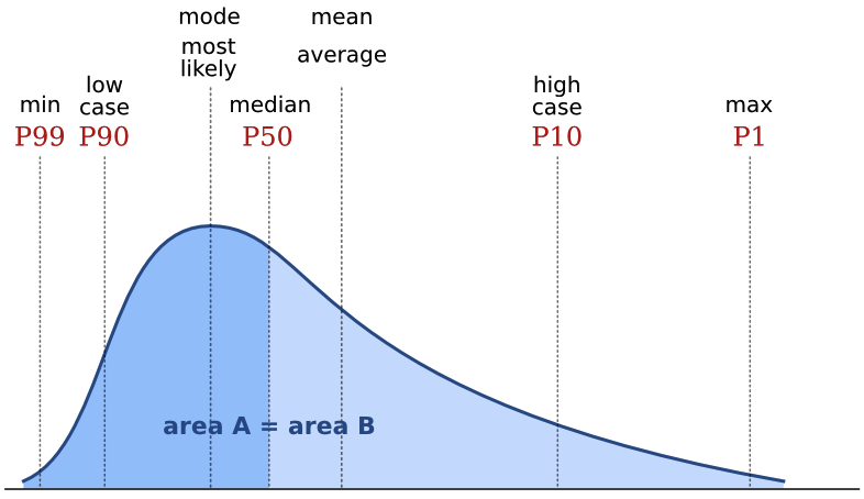
The median is the central value in the sorted data. In some ways, it's the archetypal average: the middle, with 50% of values being greater and 50% being smaller. If there is an even number of data points, then its the arithmetic mean of the middle two. In a probability distribution, the median is often called the P50. In a positively skewed distribution (the most common one in petroleum geoscience), it is larger than the mode and smaller than the mean:

Mode average

The mode, or most likely, is the most frequent result in the data. We often use it for what are called nominal data: classes or names, rather than the cardinal numbers we've been discussing up to now. For example, the name Smith is not the 'average' name in the US, as such, since most people are called something else. But you might say it's the central tendency of names. One of the commonest applications of the mode is in a simple voting system: the person with the most votes wins. If you are averaging data like facies or waveform classes, say, then the mode is the only average that makes sense. 

Honourable mentions

Most geophysicists know about the root mean square, or quadratic mean, because it's a measure of magnitude independent of sign, so works on sinusoids varying around zero, for example. 

The root mean square equation

Finally, the weighted mean is worth a mention. Sometimes this one seems intuitive: if you want to average two datasets, but they have different populations, for example. If you have a mean porosity of 19% from a set of 90 samples, and another mean of 11% from a set of 10 similar samples, then it's clear you can't simply take their arithmetic average — you have to weight them first: (0.9 × 0.21) + (0.1 × 0.14) = 0.20. But other times, it's not so obvious you need the weighted sum, like when you care about the perception of the data points

Are there other averages you use? Do you see misuse and abuse of averages? Have you ever been caught out? I'm almost certain I have, but it's too late now...

There is an even longer version of this article in the wiki. I just couldn't bring myself to post it all here. 

Are you a poet or a mathematician?

Woolly ramsMany geologists can sometimes be rather prone to a little woolliness in their language. Perhaps because you cannot prove anything in geology (prove me wrong), or because everything we do is doused in interpretation, opinion and even bias, we like to beat about the bush. A lot.

Sometimes this doesn't matter much. We're just sparing our future self from a guilty binge of word-eating, and everyone understands what we mean—no harm done. But there are occasions when a measure of unambiguous precision is called for. When we might want to be careful about the technical meanings of words like approximately, significant, and certain.

Sherman Kent was a CIA analyst in the Cold War, and he tasked himself with bringing quantitative rigour to the language of intelligence reports. He struggled (and eventually failed), meeting what he called aesthetic opposition:

Sherman Kent portraitWhat slowed me up in the first instance was the firm and reasoned resistance of some of my colleagues. Quite figuratively I am going to call them the poets—as opposed to the mathematicians—in my circle of associates, and if the term conveys a modicum of disapprobation on my part, that is what I want it to do. Their attitude toward the problem of communication seems to be fundamentally defeatist. They appear to believe the most a writer can achieve when working in a speculative area of human affairs is communication in only the broadest general sense. If he gets the wrong message across or no message at all—well, that is life.

Sherman Kent, Words of Estimative Probability, CIA Studies in Intelligence, Fall 1964

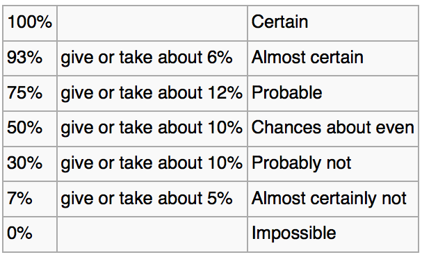
Words of estimative probabilityKent proposed using some specific words to convey specific levels of certainty (right). We have used these words in our mobile app Risk*. The only modification I made was setting P = 0.99 for Certain, and P = 0.01 for Impossible (see my remark about proving things in geology).

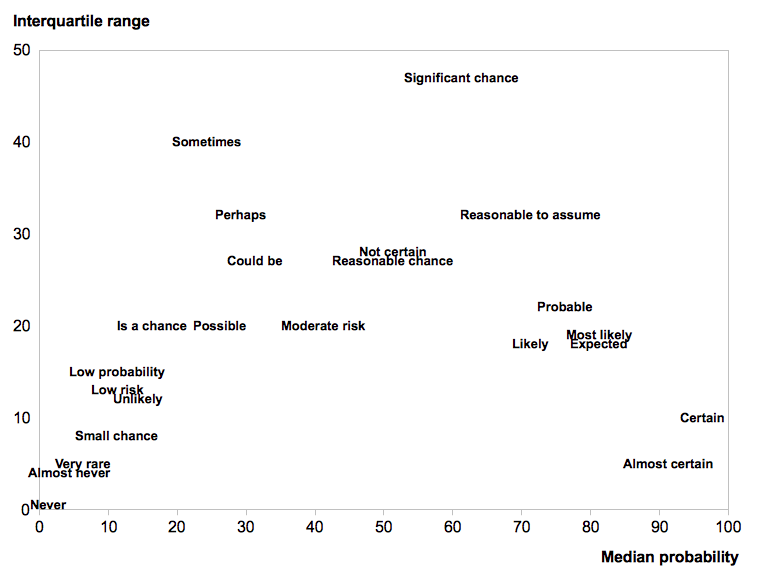
There are other schemes. Most petroleum geologists know Peter Rose's work. A common language, with some quantitative meaning, can dull the pain of prospect risking sessions. Almost certainly. Probably.

Do you use systematic descriptions of uncertainty? Do you think they help? How can we balance our poetic side of geology with the mathematical?

Reliable predictions of unlikely geology

A puzzle

Imagine you are working in a newly-accessible and under-explored area of an otherwise mature basin. Statistics show that on average 10% of structures are filled with gas; the rest are dry. Fortunately, you have some seismic analysis technology that allows you to predict the presence of gas with 80% reliability. In other words, four out of five gas-filled structures test positive with the technique, and when it is applied to water-filled structures, it gives a negative result four times out of five.

It is thought that 10% of the structures in this play are gas-filled. Your seismic attribute test is thought to be 80% reliable, because four out of five times it has indicated gas correctly. You acquire the undrilled acreage shown by the grey polygon.

You acquire some undrilled acreage—the grey polygon— then delineate some structures and perform the analysis. One of the structures tests positive. If this is the only information you have, what is the probability that it is gas-filled?

This is a classic problem of embracing Bayesian likelihood and ignoring your built-in 'representativeness heuristic' (Kahneman et al, 1982, Judgment Under Uncertainty: Heuristics and Biases, Cambridge University Press). Bayesian probability combination does not come very naturally to most people but, once understood, can at least help you see the way to approach similar problems in the future. The way the problem is framed here, it is identical to the original formulation of Kahneman et al, the Taxicab Problem. This takes place in a town with 90 yellow cabs and 10 blue ones. A taxi is involved in a hit-and-run, witnessed by a passer-by. Eye witness reliability is shown to be 80%, so if the witness says the taxi was blue, what is the probability that the cab was indeed blue? Most people go with 80%, but in fact the witness is probably wrong. To see why, let's go back to the exploration problem and look at 100 test cases.

Break it down

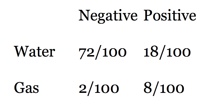
Looking at the rows in this table of outcomes, we see that there are 90 water cases and 10 gas cases. Eighty percent of the water cases test negative, and 80% of the gas cases test positive. The table shows that when we get a positive test, the probability that the test is true is not 0.80, but much less: 8/(8+18) = 0.31. In other words, a test that is mostly reliable is probably wrong when applied to an event that doesn't happen very often (a structure being gas charged). It's still good news for us, though, because a probability of discovery of 0.31 is much better than the 0.10 that we started with.

Here is Bayes' Theorem for calculating the probability P of event A (say, a gas discovery) given event B (say, a positive test in our seismic analysis):

So we can express our problem in these terms:

Are you sure about that?

This result is so counter-intuitive, for me at least, that I can't resist illustrating it with another well-known example that takes it to extremes. Imagine you test positive for a very rare disease, seismitis. The test is 99% reliable. But the disease affects only 1 person in 10 000. What is the probability that you do indeed have seismitis?

Notice that the unreliability (1%) of the test is much greater than the rate of occurrence of the disease (0.01%). This is a red flag. It's not hard to see that there will be many false positives: only 1 person in 10 000 are ill, and that person tests positive 99% of the time (almost always). The problem is that 1% of the 9 999 healthy people, 100 people, will test positive too. So for every 10 000 people tested, 101 test positive even though only 1 is ill. So the probability of being ill, given a positive test, is only about 1/101!

Lessons learned

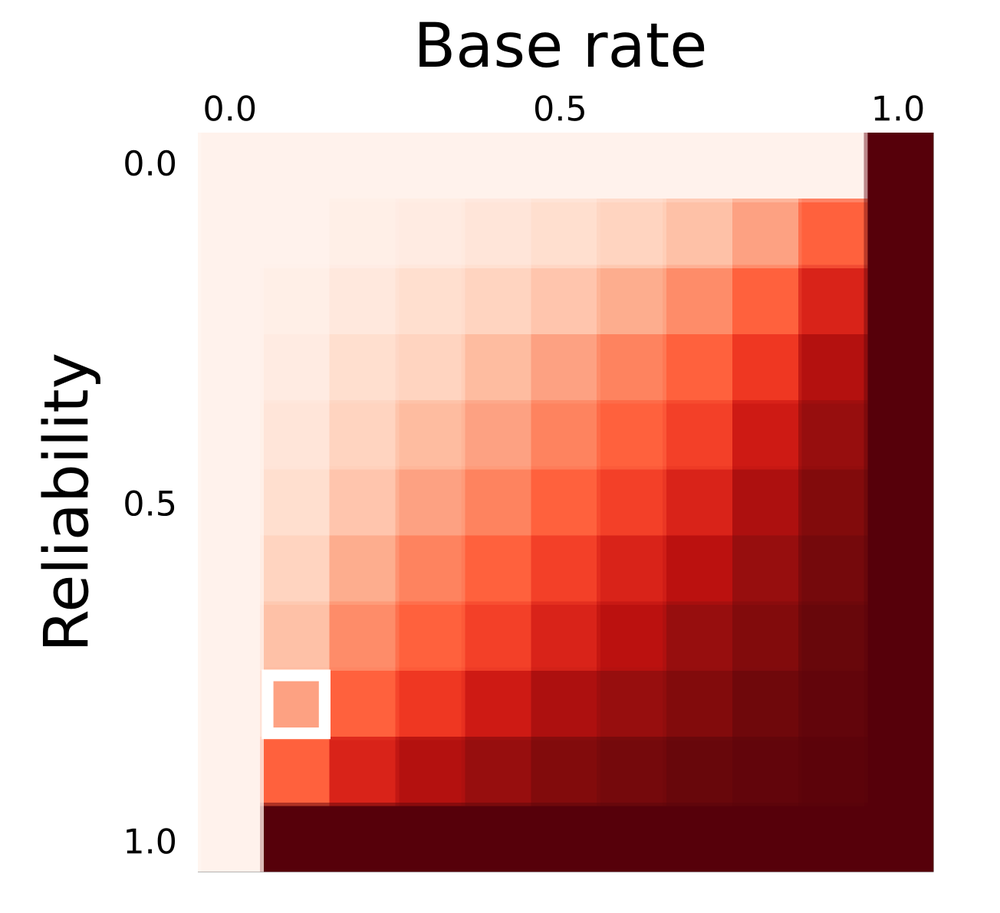
Predictive power (in Bayesian jargon, the posterior probability) as a function of test reliability and the base rate of occurrence (also called the prior probability of the event of phenomenon in question). The position of the scenario in the exploration problem is shown by the white square.

Thanks to UBC Bioinformatics for the heatmap software, heatmap.notlong.com.


Next time you confidently predict something with a seismic attribute, stop to think not only about the reliability of the test you have made, but the rate of occurrence of the thing you're trying to predict. The heatmap shows how prediction power depends on both test reliability and the occurrence rate of the event. You may be doing worse (or better!) than you think.

Fortunately, in most real cases, there is a simple mitigation: use other, independent, methods of prediction. Mutually uncorrelated seismic attributes, well data, engineering test results, if applied diligently, can improve the odds of a correct prediction. But computing the posterior probability of event A given independent observations B, C, D, E, and F, is beyond the scope of this article (not to mention this author!).

This post is a version of part of my article The rational geoscientist, The Leading Edge, May 2010

The unlikelihood of improbable events

I picked a couple of old books off my shelf last night, to sit by the fire and read something on paper for a change. I chose two classics by Darrell Huff: How To Lie With Statistics (1975 edition), and How To Take A Chance (1965 edition). They are both excellent, and the former is even still in print. The amusing story shown here (right) faces the first page.

I was a bit surprised this morning when the first thing I see, via Twitter, is this story from Reuters: wounded fox shoots its would-be (and unnamed) killer in Belarus (of all places). I thought this was quite a coincidence.

What are the chances of this being a true story, and not some sort of mistake, or hoax, or piece of folklore? At first, I thought of Bayes' theorem:

P(A|B) = \frac{P(B | A)\, P(A)}{P(B)}.

With this equation, we can calculate the probability of the story being true, given the chances of such a thing happening in the first place (slim), and the reliability of the media (pretty high). If you think the chances of a man being shot by a fox are 1 in 1000, say, and the reliability of the media is 99%, then Bayes' theroem suggests that the probability of this story being true is just 9%.

Nine percent seemed pretty low to me. Maybe I was being too hard on the media, I thought.

But then another thing I just saw yesterday was that Google News now searches archives going back over 100 years. Amazing. So I searched for fox shoots hunter, and hit Archive. And sure enough, it turns out this sort of thing happens all the time.

Shown here (left), the Wilmington Morning Star, 21 January 1981: A fox shot and killed (!) an unnamed hunter in central Yugoslavia after hitting the animal with his rifle butt. 

Another story, from the Modesto Bee of 16 November 1948, details another nasty fox-shoots-man-after-man-tries-to-wallop-injured-fox-with-rifle incident.

So, I don't know if this story is true or not, but personally I doubt it. Looking at how it has spread like rabies through the media though, I think it's fascinating how these tales become part of our experience. No-one knows where it started, and a bit of digging suggests it may even be doubtful.

How many stories like that are there in the organization where you work? And how will you question the next one you hear?