Looking ahead to SEG

SEGAM-logo-2017.jpg

The SEG Annual Meeting is coming up. Next week sees the festival of geophysics return to the global energy capital, shaken and damp but undefeated after its recent battle with Hurricane Harvey. Even though Agile will not be at the meeting this year, I wanted to point out some highlights of the week.

The Annual Meeting

The meeting will be big, as usual: 108 talk sessions, and 50 poster and e-presentation sessions. I have no idea how many presentations we're talking about but suffice to say that there's a lot. Naturally, there's a machine learning session, with the following talks:

The Geophysics Hackathon

Even though we're not at the conference, we are in Houston this weekend — for the latest edition of the Geophysics Hackathon! The focus was set to be firmly on 'machine learning', but after the hurricane, we added the theme of 'disaster recovery and mitigation'. People are completely free to choose whatever project they'd like to work on; we'll be ready to help and advise on both topics. We also have some cool gear to play with: a Dell C4130 with 4 x NVIDIA P100s, NVIDIA Jetson TX1s, Amazon Echo Dots, and a Raspberry Shake. Many, many thanks to Dell EMC and Pioneer Natural Resources and all our other sponsors:

sponsors_tight.png

If you're one of the 70 or so people coming to this event, I'm looking forward to seeing you there... if you're not, then I'm looking forward to telling you all about it next week.


Petrel User Group

icons-petrel.png

Jacob Foshee and Durwella are hosting a Petrel User Group meetup at The Dogwood, which is in midtown (not far from downtown). If you're a user of Petrel — power user or beginner, it doesn't matter — and you're interested in making the most of technology, it'd be good to see you there. Apart from anything else, you'll get to meet Jacob, who is one of those people with technology superpowers that you never know when you might need.


Rock Physics Reception

Tuesday If you've never been to the famous Rock Physics Reception, then you're missing out. It's your best shot at bumping into the luminaries of rock physics — Colin Sayers, Stefan Gelinsky, Per Avseth, Marco Perez, Bill Goodway, Tad Smith — you know the sort of thing. If the first thing you think about when you wake up in the morning is Lamé's second parameter, RSVP right now. Hurry: there are only a handful of spots left.


There's more! Don't miss:

  • The Women's Network Breakfast on Wednesday.
  • The Wiki Committee meeting on Wednesday, 8:00 am, Hilton Room 344B.
  • If you're an SEG member, you can go to any committee meeting you like! Find one that matches your interests.

If you know of any other events, please drop them in the comments!


Hooke's oolite

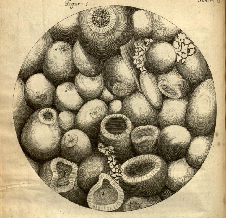
52 Things You Should Know About Rock Physics came out last week. For the first, and possibly the last, time a Fellow of the Royal Society — the most exclusive science club in the UK — drew the picture on the cover. The 353-year-old drawing was made by none other than Robert Hooke

The title page from Micrographia, and part of the dedication to Charles II. You can browse the entire book at archive.org.

The title page from Micrographia, and part of the dedication to Charles II. You can browse the entire book at archive.org.

The drawing, or rather the engraving that was made from it, appears on page 92 of Micrographia, Hooke's groundbreaking 1665 work on microscopy. In between discovering and publishing his eponymous law of elasticity (which Evan wrote about in connection with Lamé's \(\lambda\)), he drew and wrote about his observations of a huge range of natural specimens under the microscope. It was the first time anyone had recorded such things, and it was years before its accuracy and detail were surpassed. The book established the science of microscopy, and also coined the word cell, in its biological context.

Sadly, the original drawing, along with every other drawing but one from the volume, was lost in the Great Fire of London, 350 years ago almost to the day. 

Ketton stone

The drawing on the cover of the new book is of the fractured surface of Ketton stone, a Middle Jurassic oolite from central England. Hooke's own description of the rock, which he mistakenly called Kettering Stone, is rather wonderful:

I wonder if anyone else has ever described oolite as looking like the ovary of a herring?

These thoughtful descriptions, revealing a profundly learned scientist, hint at why Hooke has been called 'England's Leonardo'. It seems likely that he came by the stone via his interest in architecture, and especially through his friendsip with Christopher Wren. By 1663, when it's likely Hooke made his observations, Wren had used the stone in the façades of several Cambridge colleges, including the chapels of Pembroke and Emmanuel, and the Wren Library at Trinity (shown here). Masons call porous, isotropic rock like Ketton stone 'freestone', because they can carve it freely to make ornate designs. Rock physics in action!

You can read more about Hooke's oolite, and the geological significance of his observations, in an excellent short paper by material scientist Derek Hull (1997). It includes these images of Ketton stone, for comparison with Hooke's drawing:

Reflected light photomicrograph (left) and backscatter scanning electron microscope image (right) of Ketton Stone. Adapted from figures 2 and 3 of Hull (1997). Images are © Royal Society and used in accordance with their terms.

Reflected light photomicrograph (left) and backscatter scanning electron microscope image (right) of Ketton Stone. Adapted from figures 2 and 3 of Hull (1997). Images are © Royal Society and used in accordance with their terms.

I love that this book, which is mostly about the elastic behaviour of rocks, bears an illustration by the man that first described elasticity. Better still, the illustration is of a fractured rock — making it the perfect preface. 


References

Hall, M & E Bianco (eds.) (2016). 52 Things You Should Know About Rock Physics. Nova Scotia: Agile Libre, 134 pp.

Hooke, R (1665). Micrographia: or some Physiological Descriptions of Minute Bodies made by Magnifying Glasses, pp. 93–100. The Royal Society, London, 1665.

Hull, D (1997). Robert Hooke: A fractographic study of Kettering-stone. Notes and Records of the Royal Society of London 51, p 45-55. DOI: 10.1098/rsnr.1997.0005.

52 Things... Rock Physics

There's a new book in the 52 Things family! 

52 Things You Should Know About Rock Physics is out today, and available for purchase at Amazon.com. It will appear in their European stores in the next day or two, and in Canada... well, soon. If you can't wait for that, you can buy the book immediately direct from the printer by following this link.

The book mines the same vein as the previous volumes. In some ways, it's a volume 2 of the original 52 Things... Geophysics book, just a little bit more quantitative. It features a few of the same authors — Sven Treitel, Brian Russell, Rachel Newrick, Per Avseth, and Rob Simm — but most of the 46 authors are new to the project. Here are some of the first-timers' essays:

  • Ludmilla Adam, Why echoes fade.
  • Arthur Cheng, How to catch a shear wave.
  • Peter Duncan, Mapping fractures.
  • Paul Johnson, The astonishing case of non-linear elasticity.
  • Chris Liner, Negative Q.
  • Chris Skelt, Five questions to ask the petrophysicist.

It's our best collection of essays yet. We're very proud of the authors and the collection they've created. It stretches from childhood stories to linear algebra, and from the microscope to seismic data. There's no technical book like it. 

Supporting Geoscientists Without Borders

Purchasing the book will not only bring you profund insights into rock physics — there's more! Every sale sends $2 to Geoscientists Without Borders, the SEG charity that supports the humanitarian application of geoscience in places that need it. Read more about their important work.

It's been an extra big effort to get this book out. The project was completely derailed in 2015, as we — like everyone else — struggled with some existential questions. But we jumped back into it earlier this year, and Kara (the managing editor, and my wife) worked her magic. She loves working with the authors on proofs and so on, but she doesn't want to see any more equations for a while.

If you choose to buy the book, I hope you enjoy it. If you enjoy it, I hope you share it. If you want to share it with a lot of people, get in touch — we can help. Like the other books, the content is open access — so you are free to share and re-use it as you wish. 

Q is for Q

Quality factor, or \(Q\), is one of the more mysterious quantities of seismology. It's right up there with Lamé's \(\lambda\) and Thomsen's \(\gamma\). For one thing, it's wrapped up with the idea of attenuation, and sometimes the terms \(Q\) and 'attenuation' are bandied about seemingly interchangeably. For another thing, people talk about it like it's really important, but it often seems to be completely ignored.

A quick aside. There's another quality factor: the rock quality factor, popular among geomechnicists (geomechanics?). That \(Q\) describes the degree and roughness of jointing in rocks, and is probably related — coincidentally if not theoretically — to seismic \(Q\) in various nonlinear and probably profound ways. I'm not going to say any more about it, but if this interests you, read Nick Barton's book, Rock Quality, Seismic Velocity, Attenuation and Anistropy (2006; CRC Press) if you can afford it. 

So what is Q exactly?

We know intuitively that seismic waves lose energy as they travel through the earth. There are three loss mechanisms: scattering (elastic losses resulting from reflections and diffractions), geometrical spreading, and intrinsic attenuation. This last one, anelastic energy loss due to absorption — essentially the deviation from perfect elasticity — is what I'm trying to describe here.

I'm not going to get very far, by the way. For the full story, start at the seminal review paper entitled \(Q\) by Leon Knopoff (1964), which surely has the shortest title of any paper in geophysics. (Knopoff also liked short abstracts, as you see here.)

The dimensionless seismic quality factor \(Q\) is defined in terms of the energy \(E\) stored in one cycle, and the change in energy — the energy dissipated in various ways, such as fluid movement (AKA 'sloshing', according to Carl Reine's essay in 52 Things... Geophysics) and intergranular frictional heat ('jostling') — over that cycle:

$$ Q \stackrel{\mathrm{def}}{=} 2 \pi \frac{E}{\Delta E} $$

Remarkably, this same definition holds for any resonator, including pendulums and electronics. Physics is awesome!

Because the right-hand side of that relationship is sort of upside down — the loss is in the denominator — it's often easier to talk about \(Q^{-1}\) which is, more or less, the percentage loss of energy in a single wavelength. This inverse of \(Q\) is proportional to the attenuation coefficient. For more details on that relationship, check out Carl Reine's essay.

This connection with wavelengths means that we have to think about frequency. Because high frequencies have shorter cycles (by definition), they attenuate faster than low frequencies. You know this intuitively from hearing the beat, but not the melody, of distant music for example. This effect does not imply that \(Q\) depends on frequency... that's a whole other can of worms. (Confused yet?)

The frequency dependence of \(Q\)

It's thought that \(Q\) is roughly constant with respect to frequency below about 1 Hz, then increases with \(f^\alpha\), where \(\alpha\) is about 0.7, up to at least 25 Hz (I'm reading this in Mirko van der Baan's 2002 paper), and probably beyond. Most people, however, seem to throw their hands up and assume a constant \(Q\) even in the seismic bandwidth... mainly to make life easier when it comes to seismic processing. Attempting to measure, let alone compensate for, \(Q\) in seismic data is, I think it's fair to say, an unsolved problem in exploration geophysics.

Why is it worth solving? I think the main point is that, if we could model and measure it better, it could be a semi-independent measure of some rock properties we care about, especially velocity. Actually, I think it's even a stretch to call velocity a rock property — most people know that velocity depends on frequency, at least across the gulf of frequencies between seismic and acoustic logging tools, but did you know that velocity also depends on amplitude? Paul Johnson tells about this effect in his essay in the forthcoming 52 Things... Rock Physics book — stay tuned for more on that.

For a really wacky story about negative values of \(Q\) — which imply transmission coefficients greater than 1 (think about that) — check out Chris Liner's essay in the same book (or his 2014 paper in The Leading Edge). It's not going to help \(Q\) get any less mysterious, but it's a good story. Here's the punchline from a Jupyter Notebook I made a while back; it follows along with Chris's lovely paper:

Top: Velocity and the Backus average velocity in the E-38 well offshore Nova Scotia. Bottom: Layering-induced attenuation, or 1/Q, in the same well. Note the negative numbers! Reproduction of Liner's 2014 results in a Jupyter Notebook.

Top: Velocity and the Backus average velocity in the E-38 well offshore Nova Scotia. Bottom: Layering-induced attenuation, or 1/Q, in the same well. Note the negative numbers! Reproduction of Liner's 2014 results in a Jupyter Notebook.

Hm, I had hoped to shed some light on \(Q\) in this post, but I seem to have come full circle. Maybe explaining \(Q\) is another unsolved problem.

References

Barton, N (2006). Rock Quality, Seismic Velocity, Attenuation and Anisotropy. Florida, USA: CRC Press. 756 pages. ISBN 9780415394413.

Johnson, P (in press). The astonishing case of non-linear elasticity.  In: Hall, M & E Bianco (eds), 52 Things You Should Know About Rock Physics. Nova Scotia: Agile Libre, 2016, 132 pp.

Knopoff, L (1964). Q. Reviews of Geophysics 2 (4), 625–660. DOI: 10.1029/RG002i004p00625.

Reine, C (2012). Don't ignore seismic attenuation. In: Hall, M & E Bianco (eds), 52 Things You Should Know About Geophysics. Nova Scotia: Agile Libre, 2012, 132 pp.

Liner, C (2014). Long-wave elastic attenuation produced by horizontal layering. The Leading Edge 33 (6), 634–638. DOI: 10.1190/tle33060634.1. Chris also blogged about this article.

Liner, C (in press). Negative Q. In: Hall, M & E Bianco (eds), 52 Things You Should Know About Rock Physics. Nova Scotia: Agile Libre, 2016, 132 pp.

van der Bann, M (2002). Constant Q and a fractal, stratified Earth. Pure and Applied Geophysics 159 (7–8), 1707–1718. DOI: 10.1007/s00024-002-8704-0.

Poisson's controversial stretch-squeeze ratio

Before reading this, you might want to check out the previous post about Siméon Denis Poisson's life and career. Then come back here...


Physicists and mathematicians knew about Poisson's ratio well before Poisson got involved with it. Thomas Young described it in his 1807 Lectures on Natural Philosophy and the Mechanical Arts:

We may easily observe that if we compress a piece of elastic gum in any direction, it extends itself in other directions: if we extend it in length, its breadth and thickness are diminished.

Young didn't venture into a rigorous formal definition, and it was referred to simply as the 'stretch-squeeze ratio'.

A new elastic constant?

Twenty years later, at a time when France's scientific muscle was fading along with the reign of Napoleon, Poisson published a paper attempting to restore his slightly bruised (by his standards) reputation in the mechanics of physical materials. In it, he stated that for a solid composed of molecules tightly held together by central forces on a crystalline lattice, the stretch squeeze ratio should equal 1/2 (which is equivalent to what we now call a Poisson's ratio of 1/4). In other words, Poisson regarded the stretch-squeeze ratio as a physical constant: the same value for all solids, claiming, 'This result agrees perfectly' with an experiment that one of his colleagues, Charles Cagniard de la Tour, recently performed on brass. 

Poisson's whole-hearted subscription to the corpuscular school certainly prejudiced his work. But the notion of discovering of a new physical constant, like Newton did for gravity, or Einstein would eventually do for light, must have been a powerful driving force. A would-be singular elastic constant could unify calculations for materials soft or stiff — in contrast to elastic moduli which vary over several orders of magnitude. 

Poisson's (silly) ratio

Later, between 1850 and 1870, the physics community acquired more evidence that the stretch-squeeze ratio was different for different materials, as other materials were deformed with more reliable measurements. Worse still, de la Tour's experiments on the elasticity of brass, upon which Poisson had hung his hat, turned out to be flawed. The stretch-squeeze ratio became known as Poisson's ratio not as a tribute to Poisson, but as a way of labeling a flawed theory. Indeed, the falsehood became so apparent that it drove the scientific community towards treating elastic materials as continuous media, as opposed to an ensemble of particles.

Today we define Poisson's ratio in terms of strain (deformation), or Lamé's parameters, or the speed \(V\) of P- and S-waves:


Interestingly, if Poisson turned out to be correct, and Poisson's ratio was in fact a constant, that would mean that the number of elastic constants it would take to describe an isotropic material would be one instead of two. It wasn't until Augustin Louis Cauchy used the notion of a stress tensor to describe the state of stress at a point within a material, with its three normal stresses and three shear stresses, did the need for two elastic constants become apparent. Tensors gave the mathematical framework to define Hooke's law in three dimensions. Found in the opening chapter in any modern textbook on seismology or mechanical engineering, continuum mechanics represents a unique advancement in science set out to undo Poisson's famously false deductions backed by insufficient data.

References

Greaves, N (2013). Poisson's ratio over two centuries: challenging hypothesis. Notes & Records of the Royal Society 67, 37-58. DOI: 10.1098/rsnr.2012.0021

Editorial (2011). Poisson's ratio at 200, Nature Materials10 (11) Available online.


Deriving equations in Python

Last week I wrote about the elastic moduli, and showed the latest version of my table of equations. Here it is; click on it for a large version:

Making this grid was a bit of an exercise in itself. One could spend some happy hours rearranging things by hand; instead, I spent some (mostly) happy hours learning to use SymPy, a symbolic maths library for Python. For what it's worth, you can see my flailing in this Jupyter Notebook. Warning: it's pretty untidy.

Wrangling equations

Fortunately, SymPy is easy to get started with. Let's look at getting an expression for \(V_\mathrm{P}\) in terms of \(E\) and \(K\), given that I already have an expression in terms of \(E\) and \(\mu\), plus an expression for \(\mu\) in terms of \(E\) and \(K\).

First we import the SymPy library, set it up for nice math display in the Notebook, and initialize some parameter names:

 
>>> import sympy
>>> sympy.init_printing(use_latex='mathjax')
>>> lamda, mu, nu, E, K, rho = sympy.symbols("lamda, mu, nu, E, K, rho")

lamda is not a typo: lambda means something else in Python — it's a sort of unnamed function.

Now we're ready to define an expression. First, I'll import SymPy's own square root function for convenience. Then I define an expression for \(V_\mathrm{P}\) in terms of \(E\) and \(\mu\):

 
>>> vp_expr = sympy.sqrt((mu * (E - 4*mu)) / (rho * (E - 3*mu)))
>>> vp_expr

$$ \sqrt{\frac{\mu \left(E - 4 \mu\right)}{\rho \left(E - 3 \mu\right)}} $$

Now we can give SymPy the expression for \(\mu\) in terms of \(E\) and \(K\) and substitute:

 
>>> mu_expr = (3 * K * E) / (9 * K - E)
>>> vp_new = vp_expr.subs(mu, mu_expr)
>>> vp_new

$$\sqrt{3} \sqrt{\frac{E K \left(- \frac{12 E K}{- E + 9 K} + E\right)}{\rho \left(- E + 9 K\right) \left(- \frac{9 E K}{- E + 9 K} + E\right)}}$$

Argh, what is that?? Luckily, it's easy to simplify:

 
>>> sympy.simplify(vp_new)

$$\sqrt{3} \sqrt{\frac{K \left(E + 3 K\right)}{\rho \left(- E + 9 K\right)}}$$

That's more like it! What's really cool is that SymPy can even generate the \(\LaTeX\) code for your favourite math renderer:

 
>>> print(sympy.latex(sympy.simplify(vp_new)))
\sqrt{3} \sqrt{\frac{K \left(E + 3 K\right)}{\rho \left(- E + 9 K\right)}}

That's all there is to it!

What is the mystery X?

Have a look at the expression for  \(V_\mathrm{P}\) in terms of \(E\) and \(\lambda\):


$$\frac{\sqrt{2}}{2} \sqrt{\frac{1}{\rho} \left(E - \lambda + \sqrt{E^{2} + 2 E \lambda + 9 \lambda^{2}}\right)}$$

I find this quantity — I call it \(X\) in the big table of equations — really curious:


$$ X = \sqrt{9\lambda^2 + 2E\lambda + E^2} $$

As you can see from the similar table on Wikipedia, a similar quantity appears in expressions in terms of \(E\) and \(M\). These quantities look like elastic moduli, and even have the right units and order of magnitude as the others. If anyone has thoughts on what significance it might have, if any, or on why expressions in terms of \(E\) and \(\lambda\) or \(M\) should be so uncommonly clunky, I'm all ears. 

One last thing... I've mentioned Melvyn Bragg's wonderful BBC radio programme In Our Time before. If you like listening to the radio, try this recent episode on the life and work of Robert Hooke. Not only did he invent the study of elasticity with his eponymous law, he was also big in microscopy, describing things like the cellular structure of cork in detail (right).

All the elastic moduli

An elastic modulus is the ratio of stress (pressure) to strain (deformation) in an isotropic, homogeneous elastic material:

$$ \mathrm{modulus} = \frac{\mathrm{stress}}{\mathrm{strain}} $$

OK, what does that mean?

Elastic means what you think it means: you can deform it, and it springs back when you let go. Imagine stretching a block of rubber, like the picture here. If you measure the stress \(F/W^2\) (i.e. the pressure is force per unit of cross-sectional area) and strain \(\Delta L/L\) (the stretch as a proportion) along the direction of stretch ('longitudinally'), then the stress/strain ratio gives you Young's modulus, \(E\).

Since strain is unitless, all the elastic moduli have units of pressure (pascals, Pa), and is usually on the order of tens of GPa (billions of pascals) for rocks. 

The other elastic moduli are: 

There's another quantity that doesn't fit our definition of a modulus, and doesn't have units of pressure — in fact it's unitless —  but is always lumped in with the others: 

What does this have to do with my data?

Interestingly, and usefully, the elastic properties of isotropic materials are described completely by any two moduli. This means that, given any two, we can compute all of the others. More usefully still, we can also relate them to \(V_\mathrm{P}\), \(V_\mathrm{S}\), and \(\rho\). This is great because we can get at those properties easily via well logs and less easily via seismic data. So we have a direct path from routine data to the full suite of elastic properties.

The only way to measure the elastic moduli themselves is on a mechanical press in the laboratory. The rock sample can be subjected to confining pressures, then squeezed or stretched along one or more axes. There are two ways to get at the moduli:

  1. Directly, via measurements of stress and strain, so called static conditions.

  2. Indirectly, via sonic measurements and the density of the sample. Because of the oscillatory and transient nature of the sonic pulses, we call these dynamic measurements. In principle, these should be the most comparable to the measurements we make from well logs or seismic data.

Let's see the equations then

The elegance of the relationships varies quite a bit. Shear modulus \(\mu\) is just \(\rho V_\mathrm{S}^2\), but Young's modulus is not so pretty:

$$ E = \frac{\rho V_\mathrm{S}^2 (3 V_\mathrm{P}^2 - 4 V_\mathrm{S}^2) }{V_\mathrm{P}^2 - V_\mathrm{S}^2} $$

You can see most of the other relationships in this big giant grid I've been slowly chipping away at for ages. Some of it is shown below. It doesn't have most of the P-wave modulus expressions, because no-one seems too bothered about P-wave modulus, despite its obvious resemblance to acoustic impedance. They are in the version on Wikipedia, however (but it lacks the \(V_\mathrm{P}\) and \(V_\mathrm{S}\) expressions).

Some of the expressions for the elastic moduli and velocities — click the image to see them all in SubSurfWiki.

Some of the expressions for the elastic moduli and velocities — click the image to see them all in SubSurfWiki.

In this table, the mysterious quantity \(X\) is given by:

$$ X = \sqrt{9\lambda^2 + 2E\lambda + E^2} $$

In the next post, I'll come back to this grid and tell you how I've been deriving all these equations using Python.


Top tip... To find more posts on rock physics, click the Rock Physics tag below!

The Rock Property Catalog again

Do you like data? Data about rocks? Open, accessible data that you can use for any purpose without asking? Read on.

After writing about anisotropy back in February, and then experimenting with storing rock properties in SubSurfWiki later that month, a few things happened:

  • The server I run the wiki on — legacy Amazon AWS infrastructure — crashed, and my backup strategy turned out to be <cough> flawed. It's now running on state-of-the-art Amazon servers. So my earlier efforts were mostly wiped out... Leaving the road clear for a new experiment!
  • I came across an amazing resource called Mudrock Anisotropy, or — more appealingly — Mr Anisotropy. Compiled by Steve Horne, it contains over 1000 records of rocks, gathered from the literature. It is also public domain and carries only a disclaimer. But it's a spreadsheet, and emailing a spreadsheet around is not sustainable.
  • The Common Ground database that was built by John A. Scales, Hans Ecke and Mike Batzle at Colorado School of Mines in the late 1990s, is now defunct and has been officially discontinued, as of about two weeks ago. It contains over 4000 records, and is public domain. The trouble is, you have to restore a SQLite database to use it.

All this was pointing towards a new experiment. I give you: the Rock Property Catalog again! This time it contains not 66 rocks, but 5095 rocks. Most of them have \(V_\mathrm{P}\), \(V_\mathrm{S}\) and  \(\rho\). Many of them have Thomsen's parameters too. Most have a lithology, and they all have a reference. Looking for Cretaceous shales in North America to use as analogs on your crossplots? There's a rock for that.

As before, you can query the catalog in various ways, either via the wiki or via the web API. Let's say we want to find shales with a velocity over 5000 m/s. You have a few options:

  1. Go to the semantic search form on the wiki and type [[lithology::shale]][[vp::>5000]]
  2. Make a so-called inline query on your own wiki page (you need an account for this).
  3. Make a query via the web API with a rather long URL: http://www.subsurfwiki.org/api.php?action=ask&query=[[RPC:%2B]][[lithology::shale]][[Vp::>5000]]|%3FVp|%3FVs|%3FRho&format=jsonfm

I updated the Jupyter Notebook I published last time with a new query. It's pretty hacky. I'll work on this to produce a more robust method, with some error handling and cleaner code — stay tuned.

The database supports lots of properties, including:

  • Citation and reference
  • Description, lithology, colour (you can have pictures if you want!)
  • Location, lat/lon, basin, age, depth
  • Vp, Vs, \(\rho\), as well as \(\rho_\mathrm{dry}\) and \(\rho_\mathrm{grain}\)
  • Thomsen's \(\epsilon\), \(\delta\), and \(\gamma\)
  • Static and dynamic Young's modulus and Poisson ratio
  • Confining pressure, pore pressure, effective stress, axial stress
  • Frequency
  • Fluid, saturation type, saturation
  • Porosity, permeability, temperature
  • Composition

There is more from the Common Ground data to add, especially photographs. But for now, I'd love some feedback: is this the right set of properties? Do we need more? I want this to be useful — what kind of data and metadata would you like to see? 

I'll end with the usual appeal — I'm open to any kind of suggestions or help with this. Perhaps you can contribute new rocks, or a paper containing data? Or maybe you have some wiki skills, or can help write bots to improve the data? What can you bring? 

Introducing Bruges

bruges_rooves.png

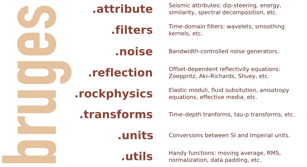
Welcome to Bruges, a Python library (previously known as agilegeo) that contains a variety of geophysical equations used in processing, modeling and analysing seismic reflection and well log data. Here's what's in the box so far, with new stuff being added every week:


Simple AVO example

VP [m/s] VS [m/s] ρ [kg/m3]
Rock 1 3300 1500 2400
Rock 2 3050 1400 2075

Imagine we're studying the interface between the two layers whose rock properties are shown here...

To compute the zero-offset reflection coefficient at zero offset, we pass our rock properties into the Aki-Richards equation and set the incident angle to zero:

 >>> import bruges as b
 >>> b.reflection.akirichards(vp1, vs1, rho1, vp2, vs2, rho2, theta1=0)
 -0.111995777064

Similarly, compute the reflection coefficient at 30 degrees:

 >>> b.reflection.akirichards(vp1, vs1, rho1, vp2, vs2, rho2, theta1=30)
 -0.0965206980095

To calculate the reflection coefficients for a series of angles, we can pass in a list:

 >>> b.reflection.akirichards(vp1, vs1, rho1, vp2, vs2, rho2, theta1=[0,10,20,30])
 [-0.11199578 -0.10982911 -0.10398651 -0.0965207 ]

Similarly, we could compute all the reflection coefficients for all incidence angles from 0 to 70 degrees, in one degree increments, by passing in a range:

 >>> b.reflection.akirichards(vp1, vs1, rho1, vp2, vs2, rho2, theta1=range(70))
 [-0.11199578 -0.11197358 -0.11190703 ... -0.16646998 -0.17619878 -0.18696428]

A few more lines of code, shown in the Jupyter notebook, and we can make some plots:


Elastic moduli calculations

With the same set of rocks in the table above we could quickly calculate the Lamé parameters λ and µ, say for the first rock, like so (in SI units),

 >>> b.rockphysics.lam(vp1, vs1, rho1), b.rockphysics.mu(vp1, vs1, rho1)
 15336000000.0 5400000000.0

Sure, the equations for λ and µ in terms of P-wave velocity, S-wave velocity, and density are pretty straightforward: 


but there are many other elastic moduli formulations that aren't. Bruges knows all of them, even the weird ones in terms of E and λ.


All of these examples, and lots of others — Backus averaging,  examples are available in this Jupyter notebook, if you'd like to work through them on your own.


Bruges is a...

It is very much early days for Bruges, but the goal is to expose all the geophysical equations that geophysicists like us depend on in their daily work. If you can't find what you're looking for, tell us what's missing, and together, we'll make it grow.

What's a handy geophysical equation that you employ in your work? Let us know in the comments!

Rock property catalog

RPC.png

One of the first things I do on a new play is to start building a Big Giant Spreadsheet. What goes in the big giant spreadsheet? Everything — XRD results, petrography, geochemistry, curve values, elastic parameters, core photo attributes (e.g. RGB triples), and so on. If you're working in the Athabasca or the Eagle Ford then one thing you have is heaps of wells. So the spreadsheet is Big. And Giant. 

But other people's spreadsheets are hard to use. There's no documentation, no references. And how to share them? Email just generates obsolete duplicates and data chaos. And while XLS files are not hard to put on the intranet or Internet,  it's hard to do it in a way that doesn't involve asking people to download the entire spreadsheet — duplicates again. So spreadsheets are not the best choice for collaboration or open science. But wikis might be...

The wiki as database

Regular readers will know that I'm a big fan of MediaWiki. One of the most interesting extensions for the software is Semantic MediaWiki (SMW), which essentially turns a wiki into a database — I've written about it before. Of course we can read any wiki page over the web, but you can query an SMW-powered wiki, which means you can, for example, ask for the elastic properties of a rock, such as this Mesaverde sandstone from Thomsen (1986). And the wiki will send you this JSON string:

{u'exists': True,
 u'fulltext': u'Mesaverde immature sandstone 3 (Kelly 1983)',
 u'fullurl': u'http://subsurfwiki.org/wiki/Mesaverde_immature_sandstone_3_(Kelly_1983)',
 u'namespace': 0,
 u'printouts': {
    u'Lithology': [{u'exists': True,
      u'fulltext': u'Sandstone',
      u'fullurl': u'http://www.subsurfwiki.org/wiki/Sandstone',
      u'namespace': 0}],
    u'Delta': [0.148],
    u'Epsilon': [0.091],
    u'Rho': [{u'unit': u'kg/m\xb3', u'value': 2460}],
    u'Vp': [{u'unit': u'm/s', u'value': 4349}],
    u'Vs': [{u'unit': u'm/s', u'value': 2571}]
  }
}

This might look horrendous at first, or even at last, but it's actually perfectly legible to Python. A little bit of data wrangling and we end up with data we can easily plot. It takes no more than a few lines of code to read the wiki's data, and construct this plot of \(V_\text{P}\) vs \(V_\text{S}\) for all the rocks I have so far put in the wiki — grouped by gross lithology:

A page from the Rock Property Catalog in Subsurfwiki.org. Very much an experiment, rocks contain only a few key properties today.

A page from the Rock Property Catalog in Subsurfwiki.org. Very much an experiment, rocks contain only a few key properties today.

If you're interested in seeing how to make these queries, have a look at this IPython Notebook. It takes you through reading the data from my embryonic catalogue on Subsurfwiki, processing the JSON response from the wiki, and making the plot. Once you see how easy it is, I hope you can imagine a day when people are publishing open data on the web, and sharing tools to query and visualize it.

Imagine it, then figure out how you can help build it!


References

Thomsen, L (1986). Weak elastic anisotropy. Geophysics 51 (10), 1954–1966. DOI 10.1190/1.1442051.