M is for Migration

One of my favourite phrases in geophysics is the seismic experiment. I think we call it that to remind everyone, especially ourselves, that this is science: it's an experiment, it will yield results, and we must interpret those results. We are not observing anything, or remote sensing, or otherwise peering into the earth. When seismic processors talk about imaging, they mean image construction, not image capture. 

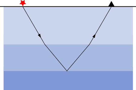
The classic cartoon of the seismic experiment shows flat geology. Rays go down, rays refract and reflect, rays come back up. Simple. If you know the acoustic properties of the medium—the speed of sound—and you know the locations of the source and receiver, then you know where a given reflection came from. Easy!

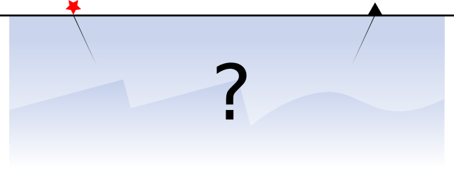But... some geologists think that the rocks beneath the earth's surface are not flat. Some geologists think there are tilted beds and faults and big folds all over the place. And, more devastating still, we just don't know what the geometries are. All of this means trouble for the geophysicist, because now the reflection could have come from an infinite number of places. This makes choosing a finite number of well locations more of a challenge. 

What to do? This is a hard problem. Our solution is arm-wavingly called imaging. We wish to reconstruct an image of the subsurface, using only our data and our sharp intellects. And computers. Lots of those.

Imaging with geometry

Agile's good friend Brian Russell wrote one of my favourite papers (Russell, 1998) — an imaging tutorial. Please read it (grab some graph paper first). He walks us through a simple problem: imaging a single dipping reflector.

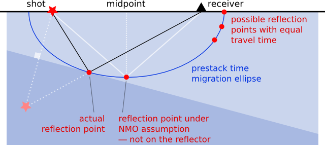
Remember that in the seismic experiment, all we know is the location of the shots and receivers, and the travel time of a sound wave from one to the other. We do not know the reflection points in the earth. If we assume dipping geology, we can use the NMO equation to compute the locus of all possible reflection points, because we know the travel time from shot to receiver. Solutions to the NMO equation — given source–receiver distance, travel time, and the speed of sound — thus give the ellipse of possible reflection points, shown here in blue:

Clearly, knowing all possible reflection points is interesting, but not very useful. We want to know which reflection point our recorded echo came from. It turns out we can do something quite easy, if we have plenty of data. Fortunately, we geophysicists always bring lots and lots of receivers along to the seismic experiment. Thousands usually. So we got data.

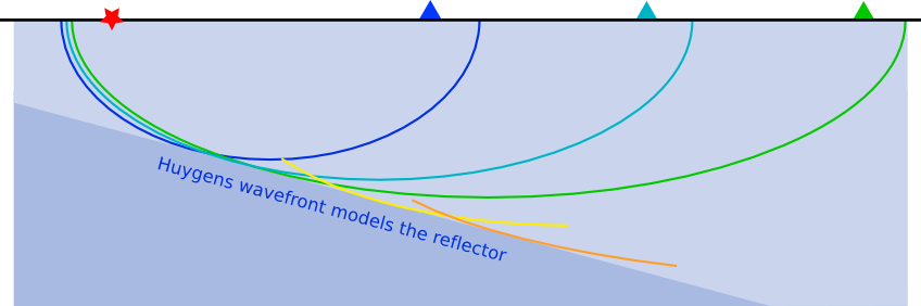
Now for the magic. Remember Huygens' principle? It says we can imagine a wavefront as a series of little secondary waves, the sum of which shows us what happens to the wavefront. We can apply this idea to the problem of the tilted bed. We have lots of little wavefronts — one for each receiver. Instead of trying to figure out the location of each reflection point, we just compute all possible reflection points, for all receivers, then add them all up. The wavefronts add constructively at the reflector, and we get the solution to the imaging problem. It's kind of a miracle. 

Try it yourself. Brian Russell's little exercise is (geeky) fun. It will take you about an hour. If you're not a geophysicist, and even if you are, I guarantee you will learn something about how the miracle of the seismic experiment. 

Reference
Russell, B (1998). A simple seismic imaging exercise. The Leading Edge 17 (7), 885–889. DOI: 10.1190/1.1438059