After reading Chris Liner's recent writings on attenuation and negative Q — both in The Leading Edge and on his blog — I've been reading up a bit on anisotropy. The idea was to stumble a little closer to writing the long-awaited Q is for Q post in our A to Z series. As usual, I got distracted...

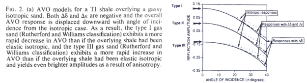
In his 1994 paper AVO in tranversely isotropic media—An overview, Blangy (now the chief geophysicist at Hess) answered a simple question: How does anisotropy affect AVO? Stigler's law notwithstanding, I'm calling his solution the Blangy equation. The answer turns out to be: quite a bit, especially if impedance contrasts are low. In particular, Thomsen's parameter δ affects the AVO response at all offsets (except zero of course), while ε is relatively negligible up to about 30°.

The key figure is Figure 2. Part (a) shows isotropic vs anisotropic Type I, Type II, and Type III responses:

Unpeeling the equation

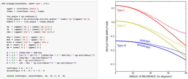
Converting the published equation to Python was straightforward (well, once Evan pointed out a typo — yay editors!). Here's a snippet, with the output (here's all of it):

For the plot below, I computed the terms of the equation separately for the Type II case. This way we can see the relative contributions of the terms. Note that the 3-term solution is equivalent to the Aki–Richards equation.

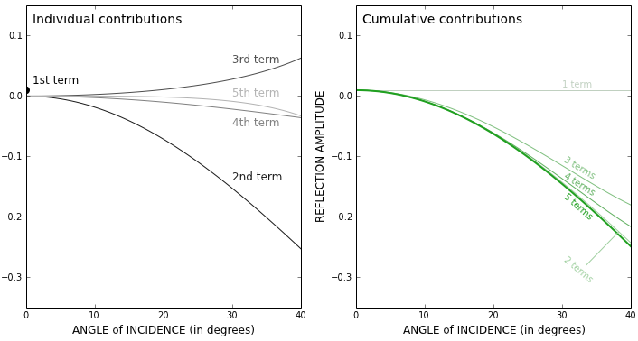
Interestingly, the 5-term result is almost the same as the 2-term approximation.

Reproducible results

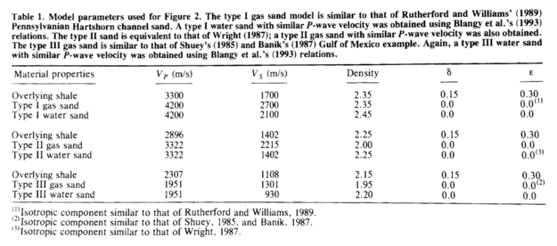
One of the other nice features of this paper — and the thing that makes it reproducible — is the unambiguous display of the data used in the models. Often, this sort of thing is buried in the text, or not available at all. A table makes it clear:

Last thought: is it just me, or is it mind-blowing that this paper is now over 20 years old?