A machine learning safety net

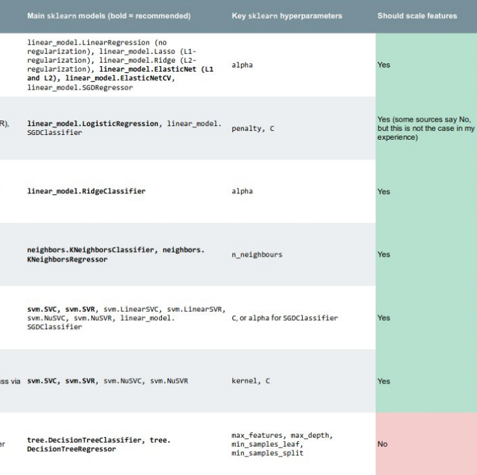
A while back, I wrote about machine learning safety measures. I was thinking about how easy it is to accidentally make terrible models (e.g. training a support vector machine on unscaled data), or misuse good models (e.g. forgetting to scale data before making a prediction). I suggested that one solution might be to make tools that help spot these kinds of mistakes:

[We should build] software to support good practice. Many of the problems I’m talking about are quite easy to catch, or at least warn about, during the training and evaluation process. Unscaled features, class imbalance, correlated features, non-IID records, and so on. Education is essential, but software can help us notice and act on them.

Introducing redflag

I’m pleased, and a bit nervous, to introduce redflag, a new Python library to help find the sorts of issues I’m describing. The vision for this tool is as a kind of safety net, or ‘entrance exam for data’ (a phrase Evan coined several years ago). It should be able to look at an array (or Pandas DataFrame), and flag potential issues, perhaps generating a report. And it should be able to sit in your Scikit-Learn pipeline, watching for issues.

The current version, 0.1.9 is still rather rough and experimental. The code is far from optimal, with quite a bit of repetition. But it does a few useful things. For example, suppose we have a DataFrame with a column, Lithology, which contains strings denoting 9 rock types (‘sandstone’, ‘limestone’, etc). We’d like to know if the classes are ‘balanced’ — present in roughly similar numbers — or not. If they are not, we will have to be careful with how we split this dataset up for our model evaluation workflow.

>>> import redflag as rf
>>> rf.imbalance_degree(df['Lithology'])
3.37859304086633
>>> rf.imbalance_ratio([df['Lithology'])
8.347368421052632

The imbalance degree, defined by Ortigosa-Hernandez et al. (2017), tells us that there are 4 minority classes (the next integer above this number), and that the imbalance severity is somewhere in the middle (3.1 would be well balanced, 3.9 would be strongly imbalanced). The simpler imbalance ratio tells us that there’s about 8 times as much of the biggest majority class as of the smallest minority class. Conclusion: depending on the size of this dataset, the class imbalance is probably not a show-stopper, but we need to pay attention.

Our dataset contains well log data. Unless they are very far apart, well log samples are usually not independent — they are correlated in depth — and this means we can’t split the data randomly in our evaluation workflow. Redflag has a function to help detect features that are correlated to themselves in this way:

>>> rf.is_correlated(df['GR'])
True

We need to be careful!

Another function, rf.wasserstein() computes the Wasserstein distance, aka the earth mover’s distance, between distributions. This can help us figure out if our data splits all have similar distributions or not — an important condition of our evaluation workflow. I’ll feed it 3 splits in which I have forgotten to scale the first feature (i.e. the first column) in the X_test dataset:

>>> rf.wasserstein([X_train, X_val, X_test])
array([[32.108,  0.025,  0.043,  0.034],
       [16.011,  0.025,  0.039,  0.057],
       [64.127,  0.049,  0.056,  0.04 ]])

The large distances in the first column are the clue that the distribution of the data in this column varies a great deal between the three datasets. Plotting the distributions make it clear what happened.

Working with sklearn

Since we’re often already working with scikit-learn pipelines, and because I don’t really want to have to remember all these extra steps and functions, I thought it would be useful to make a special redflag pipeline that runs “all the things”. It’s called rf.pipeline and it might be all you need. Here’s how to use it:

from sklearn.pipeline import make_pipeline
from sklearn.preprocessing import StandardScaler
from sklearn.svm import SVC

pipe = make_pipeline(StandardScaler(), rf.pipeline, SVC())

Here’s what this object contains:

Pipeline(steps=[('standardscaler', StandardScaler()),
                ('pipeline',
                 Pipeline(steps=[('rf.imbalance', ImbalanceDetector()),
                                 ('rf.clip', ClipDetector()),
                                 ('rf.correlation', CorrelationDetector()),
                                 ('rf.outlier', OutlierDetector()),
                                 ('rf.distributions',
                                  DistributionComparator())])),
                ('svc', SVC())])

Those redflag items in the inner pipeline are just detectors — think of them like smoke alarms — they do not change any data. Some of them acquire statistics during model fitting, then apply them during prediction. For example, the DistributionComparator learns the feature distributions from the training data, then compares the prediction data to them, to help ensure that you aren’t trying to extrapolate with your model. For example, it will warn you if you train a model on low-GR sandstones then try to predict on high-GR shales.

Here’s what happens when I fit my data with this pipeline:

These are just warnings, and it’s up to me to act on them. I can adjust detection thresholds and other aspects of the algorithms under the hood, but the goal is for redflag to wave its little flag, but not to get in the way. Apart from the warnings, this pipeline works exactly as it did before.


If this project sounds interesting or useful to you, please give it a look. The documentation is here, and contains more examples like those above. If you find bugs or want to request enhancements, there’s the GitHub Issues page. And if you use it for anything you can share, I’d love to hear how you get along!

Love Python and seismic? You need xarray

If you use Python on a regular basis, you might have noticed that Pandas is eating everything, not just things made out of bamboo.

But one thing Pandas is not useful for is 2-D or 3-D (or more-D) seismic data. Its DataFrames are implicitly two-dimensional tables, and shine when the columns represent all sorts of different quantities, e.g. different well logs. But, the really powerful thing about a DataFrame is its index. Instead of having row 0, row 1, etc, we can use an index that makes sense for the data. For example, we can use depth for the index and have row 13.1400 and row 13.2924, etc. Much easier than trying to figure out which index goes with 13.1400 metres!

Seismic data, on the other hand, does not fit comfortably in a table. But it would certainly be convenient to have real-world coordinates for the data as well as NumPy indices — maybe inline and crossline numbers, or (UTMx, UTMy) position, or the actual time position of the timeslices in milliseconds. With xarray we can.

In essence, xarray brings you Pandas-like indexing for n-dimensional arrays. Let’s see why this is useful.

Make an xarray.DataArray

The DataArray object is analogous to a NumPy array, but with the Pandas-like indexing added to each dimension via a property called coords. Furthermore, each dimension has a name.

Imagine we have a seismic volume called seismic with shape (inlines, xlines, time) and the inlines and crosslines are both numbered like 1000, 1001, 1002, etc. The time samples are 4 ms apart. All we need is an array of numbers representing inlines, another for the xlines, and another for the time samples. Then we can construct the DataArray like so:

 
import xarray as xr

il, xl, ts = seismic.shape  # seismic is a NumPy array.

inlines = np.arange(il) + 1000
xlines = np.arange(xl) + 1000
time = np.arange(ts) * 0.004

da = xr.DataArray(seismic,
                  name='amplitude',
                  coords=[inlines, xlines, time],
                  dims=['inline', 'xline', 'twt'],
                  )

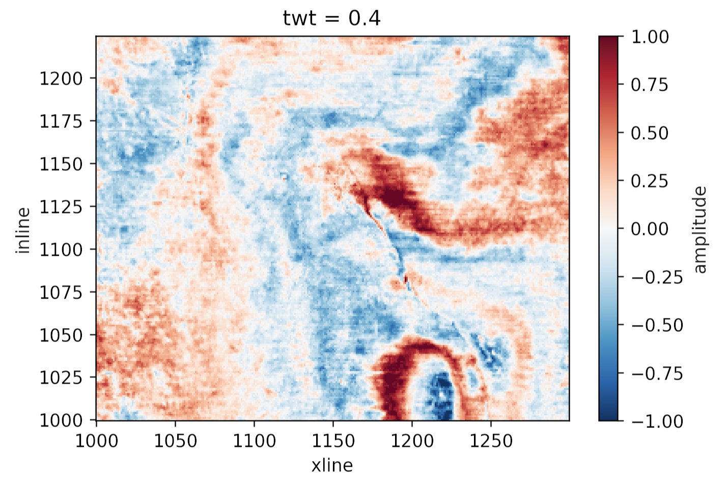
This object da has some nice superpowers. For example, we can visualize the timeslice at 400 ms with a single line:

da.sel(twt=0.400).plot()

to produce this plot:

Plotting the same thing from the NumPy array would require us to figure out which index corresponds to 400 ms, and then write at least 8 lines of matplotlib code. Nice!

What else?

Why else might we prefer this data structure over a simple NumPy array? Here are some reasons:

  • Extracting amplitude (or whatever) on a horizon. In particular, if the horizon is another DataArray with the same dims as the volume, this is a piece of cake.

  • Extracting amplitude along a wellbore (again, use the same dims for the well path).

  • Making an arbitrary line (a view not aligned with the rows/columns) is easier, because interpolation is ‘free’ with xarray.

  • Exchanging data with Pandas DataFrame objects is easy, making reading from certain formats (e.g. OpendTect horizon export, which gives you inline, xline coords, not a grid) much easier. Even better: use our library gio for this! It makes xarray objects for you.

  • If you have multiple attributes, then xarray.Dataset is a nice data structure to keep things straight. You can think of it as a dictionary of DataArray objects, but it’s a lot more than that.

  • You can store arbitrary metadata in xarray objects, so it’s easy to attach things you’d like to retain like data rights and permissions, seismic attribute parameters, data acquisition details, and so on.

  • Adding more dimensions is easy, e.g. offset or frequency, because you can just add more dims and associated coords. It can get hard to keep these straight in NumPy (was time on the 3rd or 4th axis?).

  • Taking advantage of Dask, which gives you access to parallel processing and out-of-core operations.

All in all, definitely worth a look for anyone who uses NumPy arrays to represent data with real-world coordinates.


Do you already use xarray? What kind of data does it help you with? What are your reasons? Did I miss anything from my list? Let us know in the comments!

What is an Ormsby wavelet anyway?

If you dabble in reflection seismic analysis, you probably know the Ricker wavelet. We’ve visited it a few times on this blog — Evan once showed how to make and plot one, I looked at some analytic properties of it, and we even played golf with it.

The Ricker is everywhere, but it has an important limitation — bandwidth. Its shape in the frequency domain is roughly Gaussian (below, left), which is the reason it only really has one parameter: the central frequency. This kind of spectrum is sometimes okay for older seismic surveys, especially marine data, because it matches the bandwidth reasonably. But for modern surveys, or even old land data, we often want a broader set of frequencies — more of a trapezoidal spectral shape. We need the Ormsby wavelet:

ricker-vs-ormsby.png

How to make an Ormsby wavelet

The earliest reference I can find to the Ormsby wavelet is in an article by Harold Ryan entitled, Ricker, Ormsby, Klauder, Butterworth — a choice of wavelets, in the September 1994 issue of the CSEG Recorder. It’s not clear at all who Ormsby was, other than “an aeronautical engineer”. And I don’t think anyone outside exploration geophysics knows what an Ormsby is, they just call it a ‘bandpass filter’.

Ryan helpfully provided both a time-domain analytic expression — which turns out to have four typos use the classical definiton of the sinc function — and a plot:

The equation in Ryan, and my modified Figure 3 (right). the result of the equation is in red.

The equation in Ryan, and my modified Figure 3 (right). the result of the equation is in red.

ryan_ormsby-cf-expression-2.png

This equation does not produce the wavelet (black) in the plot, however, it produces the one I’ve added in red. If you find this surprising, you shouldn’t — in my experience, it’s very common for the words and/or maths in a paper not to match its figures. [Edit: as noted above, in this case it’s because of how NumPy’s sinc function is defined; see the comment from Robert Kern, below.] We established this at the SEG Repro Zoo in 2018. If an author is not required to produce code or data, it’s not very surprising; and even if they do, the peer review system is not set up for referees to do this kind of check — apart from anything else, it’s far too onerous. But I digress.

After some fiddling around, I realized that the expression being passed to NumPy’s sinc function should be \(ft\), not \(\pi ft\). This produces a result that matches the figure almost exactly (and, counting wiggles, has the right frequency). So here’s the result of that new expression, shown in green here with the original figure (black) and the same red wavelet as above:

ryan_ormsby-cf-bruges.png

This green thing is the wavelet implemented in bruges so it’s easy to produce it; the arguments are the duration (0.4 seconds), the sample interval dt (4 ms) and the corner frequencies f (5, 10, 40, and 45 Hz respectively):

bruges.filters.ormsby(duration=0.4, dt=0.004, f=[5, 10, 40, 45])

What about other examples from the literature?

Good question! Apart from my own Python code in bruges, I did find one or two other implementations:

So it seems from this tiny experiment that only one of the implementations I found matched the figure in the Ryan article perfectly. The other wavelets are variations on the theme. Which is probably fine — after all, they are all only models for real seismic impulses — but in the interests of scientific reproducibility, I think it underscores the importance of transparent methodology and publishing your code.


Update on 9 Feb: A conversation in Software Underground revealed that Petrel’s version of the Ormsby wavelet matches the bruges implementation — but with a triangular window multiplied in (similar to how a Hamming window is multiplied into the seismic.jl version.


518px-Jupyter_logo.svg.png

I pushed my Python Jupyter Notebook to the new repro-zoo repository on GitHub. Please feel free to fork this project and add your own attempted reproductions of computational geoscience papers.

The original repro-zoo repo from the 2018 event is on SEG’s GitHub.


References

Ryan, H (1994). Ricker, Ormsby, Klauder, Butterworth — a choice of wavelets. CSEG Recorder 19 (7). Available online.

Soo-Kyung Miong, Robert R. Stewart and Joe Wong (2007). Characterizing the near surface with VSP and well logs. CREWES Research Report 19. Available online.

Three books about machine learning

I recently finished a Udemy machine learning course, and wrote on LinkedIn afterwards: “While I am no [machine learning] expert, this is one step on the way to better skills with [Python]”. So which other steps have I taken along that route to learn more about machine learning?

Here I share my thoughts on three books; two of which I have read cover to cover, and the third which I can hardly put down! When students in our machine learning class ask about books, these are the ones we recommend.

The Hundred-Page Machine Learning Book

Andriy Burkov (2019). Self-published, 141 p, ISBN 978-1-9995795-0-0. List price USD35. $30.83 at Amazon.com, £25.27 at Amazon.co.uk.

Andriy Burkov states right at the start that “[This] book is distributed on the read first, buy later principle.” That is the first time I’ve seen this in a book despite the fact you can try a car before buying or visit a house before taking out a mortgage.

This was the first book I read that is fully dedicated to machine learning. I knew a little about the topic beforehand, but wasn’t yet ready to use any machine learning algorithm at that point, so this was a perfect introduction to the what, the why and the how of machine learning. The mathematics are introduced and explained in a way that is accessible without being overwhelming, although I acknowledge that this is of course a very subjective comment.

When I turned the last page of this book (and there are a few more than 100), I was even keener to explore further, and I still refer back to this book when I want a quick summary of a machine learning concept.

Data Science from Scratch

Joel Grus (2015). O’Reilly, 311 p, ISBN 978-1-492-04113-9. List price USD 41.99 at O’Reilly. $38.85 at Amazon.com, £27.56 at Amazon.co.uk.

I read the 1st edition of this book, which uses Python 2.7 but often refers to Python 3.4; the 2nd edition (2019) uses Python 3.6 throughout.

Joel Grus, of Ten Essays on Fizz Buzz fame amongst many other achievements, has a knack of breaking problems down to their constituent parts and gracefully rebuilding a solution. While I sometimes struggled with the level of mathematics he’s comfortable with, I never felt that I couldn’t follow his journey. This book really gave me the sequence of steps in data science, and a fantastic resource to refer back to whenever an algorithm seems too opaque to me.

Introduction to Machine Learning with Python: A Guide for Data Scientists

Andreas C. Müller and Sarah Guido (2017). O’Reilly, 384 p, ISBN 978-1-449-36941-5. $40.00 at Amazon.com, £31.45 at Amazon.co.uk

At the time of writing I am halfway through this book but I’ve already gone through Chapter 2 twice: once with the book and a second time to practice with different data sets. This is symptomatic of my experience with this book so far: it’s totally addictive. Tremendously well explained, building on the power of Jupyter notebooks thanks to all the code being available on GitHub, always explaining and illustrating the effects of only the important hyperparameters in each algorithm — this is fast turning into my go-to companion for machine learning.

If you only buy one machine learning book, or don’t know where to start, this is probably the one to go with.

We all have different technical backgrounds and abilities, and as mathematics figures prominently in the implementation of all machine learning solutions, it’s not the most approachable of subjects. I’d love to hear your comments about books you would recommend to other scientists getting started in machine learning.


These prices are Amazon's discounted prices and are subject to change. The links contain a tag that earns us a small commission, but does not change the price to you. You can almost certainly buy these books elsewhere. 

The images on this page are copyright of their respective owners and are used here in accordance with fair use doctrine.

x lines of Python: Stereonets

Difficulty rating: Intermediate

A few years back I needed to plot some fracture data without specialist software, so I created an Excel spreadsheet with a polar plot and interactive widgets. But thanks to Joe Kington and his awesome mplstereonet library those days are over. Today I want to share with you how to plot two fracture sets on an equal area Schmidt plot with mplstereonet.

Here's what we're going to do — and in only 10 lines of Python:

  1. Load the data from a CSV file.
  2. Create a stereonet with grid lines.
  3. Loop over fracture sets and plot each in a different colour.
  4. Add some statistics for each set.

For data we'll use Irene Wallis's fantastic open-source project fractoolbox repo, which includes some data — as well as some notebooks that go beyond what we will do here.

This results in the plot shown here, where each fracture is plotted as a point representing the pole of the fracture plane.

We see that not counting the imports, we can make this simple plot with as a few as 10 lines of code while still retaining some flexibility to refactor this code. The accompanying notebook also shows how to use ipywidgets to make the plot interactive.

stereonet_example.jpg

That’s it! There’s more in the Notebook — check out the links below. If you get some beautiful plots out of your data, share them in the Software Underground or on Twitter. Have fun!

GitHub    See the Notebook on GitHub

Binder    Run the Notebook in MyBinder

x lines of Python: contour maps

Difficulty rating: EASY

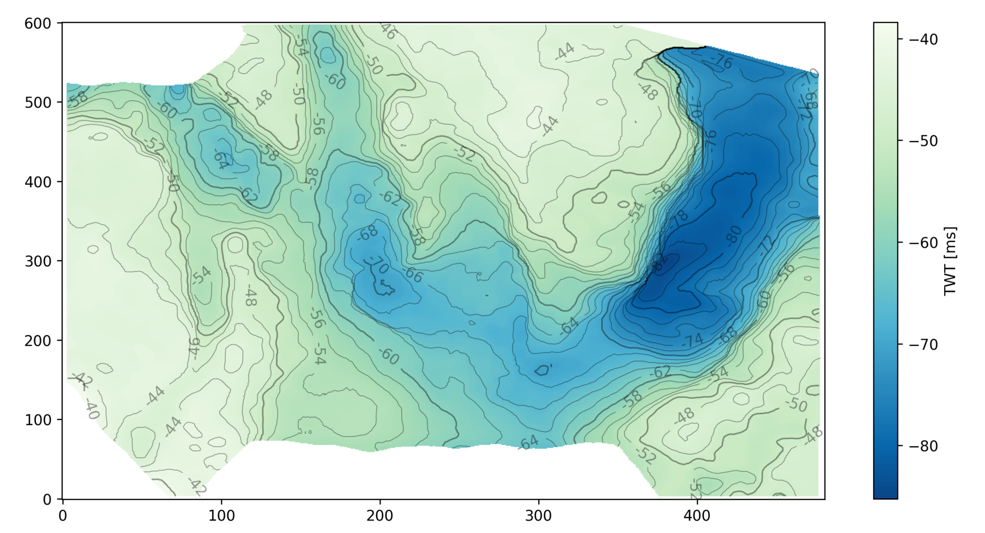
Following on from the post a couple of weeks ago about colourmaps, I wanted to poke into contour maps a little more. Ostensibly, making a contour plot in matplotlib is a one-liner:

plt.contour(data)

But making a contour plot look nice takes a little more work than most of matplotlib's other plotting functions. For example, to change the contour levels you need to make an array containing the levels you want... another line of code. Adding index contours needs another line. And then there's all the other plotty stuff.

Here's what we'll do:

  1. Load the data from a binary NumPy file.
  2. Check the data looks OK.
  3. Get the min and max values from the map.
  4. Generate the contour levels.
  5. Make a filled contour map and overlay contour lines.
  6. Make a map with index contours and contour labels.

The accompanying notebook sets out all the code you will need. You can even run the code right in your browser, no installation required.

Here's the guts of the notebook:

 
import numpy as np
import matplotlib.pyplot as plt

seabed = np.load('../data/Penobscot_Seabed.npy')
seabed *= -1
mi, ma = np.floor(np.nanmin(seabed)), np.ceil(np.nanmax(seabed))
step = 2
levels = np.arange(10*(mi//10), ma+step, step)
lws = [0.5 if level % 10 else 1 for level in levels]

# Make the plot
fig = plt.figure(figsize=(12, 8))
ax = fig.add_subplot(1,1,1)
im = ax.imshow(seabed, cmap='GnBu_r', aspect=0.5, origin='lower')
cb = plt.colorbar(im, label="TWT [ms]")
cb.set_clim(mi, ma)
params = dict(linestyles='solid', colors=['black'], alpha=0.4)
cs = ax.contour(seabed, levels=levels, linewidths=lws, **params)
ax.clabel(cs, fmt='%d')
plt.show()

This produces the following plot:

my_map.png

Why Python beats MATLAB for geophysics

MATLAB — the scientific computing environment which includes a programming language — is amazing. It has probably done as much for the development of new geophysical methods, and for the teaching and learning of geophysics, as any other tool or language. A purely anecdotal assertion, but it's rare to meet a geophysicist who has not at least dabbled in MATLAB, and it is used daily in geophysics labs and classrooms. Geophysics <3 MATLAB.

It's easy to see why — MATLAB definitely has some advantages.

Advantages of MATLAB

  • Matrices. MATLAB implicitly treats arrays as matrices (the name means 'matrix laboratory'). As a result, notation is quite intuitive for mathematicians. For example, a*b means standard matrix multiplication, the dot product. (Slightly confusingly, to get Python-style element-wise multiplication, add a dot: a.*b).
  • Lots of functions. MATLAB has been around for over 30 years, so there are many, many useful functions. Find them either in the core product, in one of the toolboxes, or in MATLAB Central.
  • Simulink. This block-based system design and simulation engine is much-loved by engineers. It allows users to model physical systems in an intuitive, graphical environment.
  • Easy to install. The MATLAB environment is a desktop application, so it is instantly familiar and can be managed under the same processes other software in your machine or organization is managed.
  • MATLAB is widespread in academia. Thanks to one of those generous schemes where software corporations give free software to universities, just because they're awesome and definitely not for any other reason, students and profs have easy and free access to MATLAB. Outside academia, however, you're looking at tens of thousands of dollars.

So far so good, but it's time for geophysics to switch to Python. On the face of it, the language has a lot in common with MATLAB: they're both easy to learn, and both have broad ecosystems that make things like image processing, statistics, and signal processing easy. But Python has some special features that make it a fantastic platform for scientific computing...

Advantages of Python

  • Free and open. Thanks to one of those generous schemes where people make software and let anyone use it for any purpose for free, Python is free! Not only is it free of charge, you are free to inspect and modify the code. Open is awesome. (There are other free alternatives to MATLAB, notably GNU Octave and SciLab.)
  • General purpose. One of the things I love about Python is its flexibility. You can use it in the shell on microtasks, or interactively, or in scripts, or to write server software, or to build enterprise software with GUIs.
  • Namespaces. Everything in MATLAB lives in the main namespace, whereas Python keeps things inherently modular. To access NumPy, say, you have to import it and then use its namespace to get at its contents: numpy.ndarray([1, 2, 3]). This has various advantages, including flexibility, readability, learnability, and portability.
  • Introspection. A powerful idea in Python, introspection means that you (or your code) can see inside every module, class, and function. You can use access private variables, or write code that 'knows' about other objects' interfaces.
  • Portable. You can run your Python code on any architecture, whereas to run MATLAB code you either need all the MATLAB licenses the software uses, or another pricey toolbox to make executables.
  • Popular. Python is the 7th most popular tag in Stack Overflow, whereas MATLAB is the 58th. While programming is not a popularity contest, think of your career, or the careers of your students. Once they graduate, Python will serve them better than MATLAB. There are over 300 jobs for Pythonistas on Stack Overflow Jobs right now. MATLAB jobs? Nine.

So there you have it. It's time to switch to Python. If you're new to programming, there's no contest. I suppose if you're productive in MATLAB, and have access to all the toolboxes, then admittedly it's hard to say you should switch.

But I'll still say it.


I was inspired to write this post after talking to a geophysicist about using programming languages in the classroom, and by the lists in this nice post on pyzo.org. It would be interesting to hear what you use in the classroom — as an instructor or as a student. I know geophysics is being taught with the help of MATLAB (in many places), Java (e.g. at Colorado School of Mines), Mathematica (e.g. by Chris Liner). I wonder if there's anyone using JavaScript, which wouldn't be a terrible choice. Or C++? Or Fortran?? Let us know in the comments!