x lines of Python: Stereonets

Difficulty rating: Intermediate

A few years back I needed to plot some fracture data without specialist software, so I created an Excel spreadsheet with a polar plot and interactive widgets. But thanks to Joe Kington and his awesome mplstereonet library those days are over. Today I want to share with you how to plot two fracture sets on an equal area Schmidt plot with mplstereonet.

Here's what we're going to do — and in only 10 lines of Python:

1. Load the data from a CSV file.
2. Create a stereonet with grid lines.
3. Loop over fracture sets and plot each in a different colour.
4. Add some statistics for each set.

For data we'll use Irene Wallis's fantastic open-source project fractoolbox repo, which includes some data — as well as some notebooks that go beyond what we will do here.

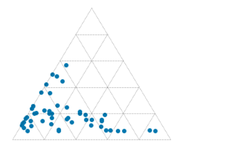
This results in the plot shown here, where each fracture is plotted as a point representing the pole of the fracture plane.

We see that not counting the imports, we can make this simple plot with as a few as 10 lines of code while still retaining some flexibility to refactor this code. The accompanying notebook also shows how to use ipywidgets to make the plot interactive.

That’s it! There’s more in the Notebook — check out the links below. If you get some beautiful plots out of your data, share them in the Software Underground or on Twitter. Have fun!

   See the Notebook on GitHub

   Run the Notebook in MyBinder

x lines of Python: static basemaps with contextily

Difficulty rating: Beginner

Something that is often useful in planning is to have a basemap of the area in which you have data or an interest. This can be made using a number of different tools, up to and including full-fledged GIS software, but we will use Contextily for a quick static basemap using Python. Installation is as simple as using conda install contextily or pip install contextily.

The steps that we want to take are the following, expressed in plain English, each of which will roughly be one line of code:

1. Get a source for our basemap (placenames and similar things)
2. Get a source for our geological map
3. Get the location that we would like to map
4. Plot the location with our geological data
5. Add the basemap to our geological map
6. Add the attribution for both maps
7. Plot our final map

We will start with the imports, which as usual do not count:

import contextily as ctx
import matplotlib.pyplot as plt

Contextily has a number of built-in providers of map tiles, which can be accessed using the ctx.providers dictionary. This is nested, with some providers offering multiple tiles. An example is the ctx.providers.OpenStreetMap.Mapnik provider, which contains the following:

{'url': 'https://{s}.tile.openstreetmap.org/{z}/{x}/{y}.png',
 'max_zoom': 19,
 'attribution': '(C) OpenStreetMap contributors',
 'name': 'OpenStreetMap.Mapnik'}

The most important parameter in the dictionary for each provider is the url. These are of the form example.com/{z}/{x}/{y}.png. The {z} is the zoom level, while {x} and {y} relate to the latitude and longitude of a given tile, respectively. Note that these are the same as those used by interactive Slippy maps; contextily just downloads them as a single static image.

The easiest is to use one of these providers, but we can also define our own provider, using the above pattern for the URL. For geological data, the Macrostrat project is a great resource, especially because they have a tileserver supplying some detail. Their tileserver can be added using

geology_tiles = 'https://tiles.macrostrat.org/carto/{z}/{x}/{y}.png'

We also need a place to map. Contextily has a geocoder that can return the tiles covering a given location. It uses OpenStreetMap, so anything that is present there is useable as a location. This includes countries (e.g. 'Paraguay'), provinces/states ('Nova Scotia'), cities ('Lubumbashi'), and so on.

We will use Nova Scotia as our area of interest, as well as giving our desired map tiles. We can also use .plot() on the Place object to get a look at it immediately, using that basemap.

ctx.Place('Nova Scotia', source=ctx.providers.CartoDB.Positron).plot()

The Positron style from Carto for Nova Scotia.

We'll use a different basemap though:

basemap = ctx.providers.Stamen.Toner

We can create the Place with our desired source — geology_tiles in this case — and then plot this on the basemap with some transparency. We will also add an attribution, since we need to credit MacroStrat.

place = ctx.Place('Nova Scotia', source=geology_tiles)

base_ax = place.plot()
ctx.add_basemap(ax=base_ax, source=basemap, alpha=0.5)
text = basemap.attribution + ' | Geological data: MacroStrat.org (CC-BY)'
ctx.add_attribution(ax=base_ax, text=text)

Finally, after a plt.show() call, we get the following:

Obviously this is still missing some important things, like a proper legend, but as a quick overview of what we can expect in a given area, it is a good approach. This workflow is probably better suited for general location maps.

Contextily also plays well with geopandas, allowing for an easy locality map of a given GeoDataFrame. Check out the accompanying Notebook for an example.

 Run the accompanying notebook in MyBinder

x lines of Python: Loading images

Difficulty rating: Beginner

We'd often like to load images into Python. Once loaded, we might want to treat them as images, for example cropping them, saving in another format, or adjusting brightness and contrast. Or we might want to treat a greyscale image as a two-dimensional NumPy array, perhaps so that we can apply a custom filter, or because the image is actually seismic data.

This image-or-array duality is entirely semantic — there is really no difference between images and arrays. An image is a regular array of numbers, or, in the case of multi-channel rasters like full-colour images, a regular array of several numbers: one for each channel. So each pixel location in an RGB image contains 3 numbers:

In general, you can go one of two ways with images:

1. Load the image using a library that 'knows about' (i.e. uses language related to) images. The preeminent tool here is pillow (which is a fork of the grandparent of all Python imaging solutions, PIL).
2. Load the image using a library that knows about arrays, like matplotlib or scipy. These wrap PIL, making it a bit easier to use, but potentially losing some options on the way.

The Jupyter Notebook accompanying this post shows you how to do both of these things. I recommend learning to use some of PIL's power, but knowing about the easier options too.

Here's the way I generally load an image:

from PIL import Image
im = Image.open("my_image.png")

(One strange thing about pillow is that, while you install it with pip install pillow, you still actually import and use PIL in your code.) This im is an instance of PIL's Image class, which is a data structure especially for images. It has some handy methods, like im.crop(), im.rotate(), im.resize(), im.filter(), im.quantize(), and lots more. Doing some of these operations with NumPy arrays is fiddly — hence PIL's popularity.

But if you just want your image as a NumPy array:

import numpy as np
arr = np.array(im)

Note that arr is a 3-dimensional array, the dimensions being row, column, channel. You can go off with arr and do whatever you need, then cast back to an Image with Image.fromarray(arr).

All this stuff is demonstrated in the Notebook accompanying this post, or you can use one of these links to run it right now in your browser:

  Run the accompanying notebook in MyBinder

---

Other posts about images:

• How to choose an image format (2012)
• When to use vectors not rasters (2012)
• Images as data (2016)
• Save the samples (2014)
• B is for bit depth (2011)

x lines of Python: Physical units

Difficulty rating: Intermediate

Have you ever wished you could carry units around with your quantities — and have the computer figure out the best units and multipliers to use?

pint is a nice, compact library for doing just this, handling all your dimensional analysis needs. It can also detect units from strings. We can define our own units, it knows about multipliers (kilo, mega, etc), and it even works with numpy and pandas.

To use it in its typical mode, we import the library then instantiate a UnitRegistry object. The registry contains lots of physical units:

import pint
units = pint.UnitRegistry()
thickness = 68 * units.m

Now thickness is a Quantity object with the value <Quantity(68, 'meter')>, but in Jupyter we see a nice 68 meter (as far as I know, you're stuck with US spelling).

Let's make another quantity and multiply the two:

area = 60 * units.km**2
volume = thickness * area

This results in volume having the value <Quantity(4080, 'kilometer ** 2 * meter')>, which pint can convert to any units you like, as long as they are compatible:

>>> volume.to('pint')
8622575788969.967 pint

More conveniently still, you can ask for 'compact' units. For example, volume.to_compact('pint') returns 8.622575788969966 terapint. (I guess that's why we don't use pints for field volumes!)

There are lots and lots of other things you can do with pint; some of them — dealing with specialist units, NumPy arrays, and Pandas dataframes — are demonstrated in the Notebook accompanying this post. You can use one of these links to run this right now in your browser if you like:

  Run the accompanying notebook in MyBinder

  Run the notebook in Google Colaboratory (note the install cell at the beginning)

That's it for pint. I hope you enjoy using it in your scientific computing projects. If you have your own tips for handling units in Python, let us know in the comments!

---

There are some other options for handling units in Python:

• quantities, which handles uncertainties without also needing the uncertainties package.
• astropy.units, part of the large astropy project, is popular among physicists.

x lines of Python: Ternary diagrams

Difficulty rating: beginner-friendly

(I just realized that calling the more approachable tutorials ‘easy’ is perhaps not the most sympathetic way to put it. But I think this one is fairly approachable.)

If you’re new to Python, plotting is a great way to get used to data structures, and even syntax, because you get immediate visual feedback. Plots are just fun.

Data loading

The first thing is to load the data, which is contained in a Google Sheets spreadsheet. If you make a sheet public, it’s easy to make a URL that provides a CSV. Happily, the Python data management library pandas can read URLs directly, so loading the data is quite easy — the only slightly ugly thing is the long URL:

    import pandas as pd
    uid = "1r7AYOFEw9RgU0QaagxkHuECvfoegQWp9spQtMV8XJGI"
    url = f"https://docs.google.com/spreadsheets/d/{uid}/export?format=csv"
    df = pd.read_csv(url) 

This dataset contains results from point-counting 51 shallow marine sandstones from the Eocene Sobrarbe Formation. We’re going to plot normalized volume percentages of quartz grains, detrital carbonate grains, and undifferentiated matrix. Three parameters? Two degrees of freedom? Let’s make a ternary plot!

Data exploration

Once you have the data in pandas, and before getting to the triangular stuff, we should have a look at it. Seaborn, a popular statistical plotting library, has a nifty ‘pairplot’ which plots the numerical parameters against each other to help reveal patterns in the data. On the diagonal, it shows kernel density estimations to reveal the distribution of each property:

    import seaborn as sns
    vars = ['Matrix', 'Quartz', 'Carbonate', 'Bioclasts', 'Authigenic']
    sns.pairplot(df, vars=vars, hue='Facies Association')

Normalization is fairly straightforward. For each column, e.g. df['Carbonate'], we make a new column, e.g. df['C'], which is normalized to the sum of the three components, given by df[cols].sum(axis=1):

cols = ['Carbonate', 'Quartz', 'Matrix']
for col in cols:
    df[col[0]] = df[col] * 100 / df[cols].sum(axis=1)

The ternary plot

For the ternary plot itself I’m using the python-ternary library, which is pretty hands-on in that most plots take quite a bit of code. But the upside of this is that you can do almost anything you want. (Theres one other option for Python, the ever-reliable plotly, and there’s a solid-looking package for R too in ggtern.)

We just need a few lines of plotting code (left) to pull a ternary diagram (right) together.

    fig, tax = ternary.figure(scale=100)
    fig.set_size_inches(5, 4.5)

    tax.scatter(df[['M', 'Q', 'C']].values)
    tax.gridlines(multiple=20)
    tax.get_axes().axis('off')

But here you see what I mean about this being quite a low-level library: each element of the plot has to be added explicitly. So if we want axis labels, titles, and other annotations, we need more code… all of which is laid out in the accompanying notebook. You can download this from GitHub, or run it right now, right in your browser, with these links:

  Run the accompanying notebook in MyBinder

  Run the notebook in Google Colaboratory (note you need to install python-ternary)

Give it a go, and have fun making your own ternary plots in Python! Share them on LinkedIn or Twitter.

Quartz, carbonate and matrix quantities (normalized to 100%) for 51 calcareous sandstones from the Eocene Sobrarbe Formation. The ternary plot was made with python-ternary library for Python and matplotlib.

x lines of Python: Gridding map data

Difficulty rating: moderate.

Welcome to the latest in the X lines of Python series. You probably thought it had died, gawn to ‘eaven, was an x-series. Well, it’s back!

Today we’re going to fit a regularly sampled surface — a grid — to an irregular set of points in (x, y) space. The points represent porosity, measured in volume percent.

Here’s what we’re going to do; it all comes to only 9 lines of code!

1. Load the data from a text file (needs 1 line of code).

2. Compute the extents and then the coordinates of the new grid (2 lines).

3. Make a radial basis function interpolator using SciPy (1 line).

4. Perform the interpolation (1 line).

5. Make a plot (4 lines).

As usual, there’s a Jupyter Notebook accompanying this blog post, and you can run it right now without installing anything.

Run the accompanying notebook in MyBinder

Run the notebook in Google Colaboratory

Just the juicy bits

The notebook goes over the workflow in a bit more detail — with more plots and a few different ways of doing the interpolation. For example, we try out triangulation and demonstrate using scikit-learn’s Gaussian process model to show how we might use kriging (turns out kriging was machine learning all along!).

If you don’t have time for all that, and just want the meat of the notebook, here it is:

import numpy as np
import pandas as pd
import matplotlib.pyplot as plt
from scipy.interpolate import Rbf

# Load the data.
df = pd.read_csv('../data/ZoneA.dat',
                 sep=' ',
                 header=9,
                 usecols=[0, 1, 2, 3],
                 names=['x', 'y', 'thick', 'por']
                )

# Build a regular grid with 500-metre cells.
extent = x_min, x_max, y_min, y_max = [df.x.min()-1000, df.x.max()+1000,
                                       df.y.min()-1000, df.y.max()+1000]
grid_x, grid_y = np.mgrid[x_min:x_max:500, y_min:y_max:500]

# Make the interpolator and do the interpolation.
rbfi = Rbf(df.x, df.y, df.por)
di = rbfi(grid_x, grid_y)

# Make the plot.
plt.figure(figsize=(15, 15))
plt.imshow(di.T, origin="lower", extent=extent)
cb = plt.scatter(df.x, df.y, s=60, c=df.por, edgecolor='#ffffff66')
plt.colorbar(cb, shrink=0.67)
plt.show()

This results in the following plot, in which the points are the original data, plotted with the same colourmap as the surface itself (so they should be the same colour, more or less, as their background).

x lines of Python: contour maps

Difficulty rating: EASY

Following on from the post a couple of weeks ago about colourmaps, I wanted to poke into contour maps a little more. Ostensibly, making a contour plot in matplotlib is a one-liner:

plt.contour(data)

But making a contour plot look nice takes a little more work than most of matplotlib's other plotting functions. For example, to change the contour levels you need to make an array containing the levels you want... another line of code. Adding index contours needs another line. And then there's all the other plotty stuff.

Here's what we'll do:

1. Load the data from a binary NumPy file.
2. Check the data looks OK.
3. Get the min and max values from the map.
4. Generate the contour levels.
5. Make a filled contour map and overlay contour lines.
6. Make a map with index contours and contour labels.

The accompanying notebook sets out all the code you will need. You can even run the code right in your browser, no installation required.

Here's the guts of the notebook:

import numpy as np
import matplotlib.pyplot as plt

seabed = np.load('../data/Penobscot_Seabed.npy')
seabed *= -1
mi, ma = np.floor(np.nanmin(seabed)), np.ceil(np.nanmax(seabed))
step = 2
levels = np.arange(10*(mi//10), ma+step, step)
lws = [0.5 if level % 10 else 1 for level in levels]

# Make the plot
fig = plt.figure(figsize=(12, 8))
ax = fig.add_subplot(1,1,1)
im = ax.imshow(seabed, cmap='GnBu_r', aspect=0.5, origin='lower')
cb = plt.colorbar(im, label="TWT [ms]")
cb.set_clim(mi, ma)
params = dict(linestyles='solid', colors=['black'], alpha=0.4)
cs = ax.contour(seabed, levels=levels, linewidths=lws, **params)
ax.clabel(cs, fmt='%d')
plt.show()

This produces the following plot:

x lines of Python: Let's play golf!

Normally in the x lines of Python series, I'm trying to do something useful in as few lines of code as possible, but — and this is important — without sacrificing clarity. Code golf, on the other hand, tries solely to minimize the number of characters used, and to heck with clarity. This might, and probably will, result in rather obfuscated code.

So today in x lines, we set x = 1 and see what kind of geophysics we can express. Follow along in the accompanying notebook if you like.

A Ricker wavelet

One of the basic building blocks of signal processing and therefore geophysics, the Ricker wavelet is a compact, pulse-like signal, often employed as a source in simulation of seismic and ground-penetrating radar problems. Here's the equation for the Ricker wavelet:

$$ A = (1-2 \pi^2 f^2 t^2) e^{-\pi^2 f^2 t^2} $$

where \(A\) is the amplitude at time \(t\), and \(f\) is the centre frequency of the wavelet. Here's one way to translate this into Python, more or less as expressed on SubSurfWiki:

import numpy as np 
def ricker(length, dt, f):
    """Ricker wavelet at frequency f Hz, length and dt in seconds.
    """
    t = np.arange(-length/2, length/2, dt)
    y = (1.0 - 2.0*(np.pi**2)*(f**2)*(t**2)) * np.exp(-(np.pi**2)*(f**2)*(t**2))
    return t, y

That is alredy pretty terse at 261 characters, but there are lots of obvious ways, and some non-obvious ways, to reduce it. We can get rid of the docstring (the long comment explaining what the function does) for a start. And use the shortest possible variable names. Then we can exploit the redundancy in the repeated appearance of \(\pi^2f^2t^2\)... eventually, we get to:

def r(l,d,f):import numpy as n;t=n.arange(-l/2,l/2,d);k=(n.pi*f*t)**2;return t,(1-2*k)/n.exp(k)

This weighs in at just 95 characters. Not a bad reduction from 261, and it's even not too hard to read. In the notebook accompanying this post, I check its output against the version in our geophysics package bruges, and it's legit:

The 95-character Ricker wavelet in green, with the points computed by the function in BRuges.

What else can we do?

In the notebook for this post, I run through some more algorithms for which I have unit-tested examples in bruges:

• The Ormsby wavelet, reduced from 1545 characters in bruges to 168 characters. (Not bad, considering it took me 111 characters just to express the mathematical equation in the wiki!)
• The 4-term Aki-Richards equation, weighing in at only 179 characters (9.8% of the 1828 characters in bruges).
• The exact Zoeppritz solution for a PP reflection, at 386 characters.

To give you some idea of why we don't normally code like this, here's what the Aki–Richards solution looks like:

def r(a,c,e,b,d,f,t):import numpy as n;w=f-e;x=f+e;y=d+c;p=n.pi*t/180;s=n.sin(p);return w/x-(y/a)**2*w/x*s**2+(b-a)/(b+a)/n.cos((p+n.arcsin(b/a*s))/2)**2-(y/a)**2*(2*(d-c)/y)*s**2

A bit hard to debug! But there is still some point to all this — I've found I've had to really understand Python's order of mathematical operations, and find different ways of doing familiar things. Playing code golf also makes you think differently about repetition and redundancy. All good food for developing the programming brain.

Do have a play with the notebook, which you can even run in Microsoft Azure, right in your browser! Give it a try. (You'll need an account to do this. Create one for free.)

---

Many thanks to Jesper Dramsch and Ari Hartikainen for helping get my head into the right frame of mind for this silliness!

x lines of Python: load curves from LAS

Welcome to the latest x lines of Python post, in which we have a crack at some fundamental subsurface workflows... in as few lines of code as possible. Ideally, x < 10.

We've met curves once before in the series — in the machine learning edition, in which we cheated by loading the data from a CSV file. Today, we're going to get it from an LAS file — the popular standard for wireline log data.

Just as we previously used the pandas library to load CSVs, we're going to save ourselves a lot of bother by using an existing library — lasio by Kent Inverarity. Indeed, we'll go even further by also using Agile's library welly, which uses lasio behind the scenes.

The actual data loading is only 1 line of Python, so we have plenty of extra lines to try something more ambitious. Here's what I go over in the Jupyter notebook that goes with this post:

1. Load an LAS file with lasio.
2. Look at its header.
3. Look at its curve data.
4. Inspect the curves as a pandas DataFrame.
5. Load the LAS file with welly.
6. Look at welly's Curve objects.
7. Plot part of a curve.
8. Smooth a curve.
9. Export a set of curves as a matrix.
10. BONUS: fix some broken things in the file header.

Each one of those steps is a single line of Python. Together, I think they cover many of the things we'd like to do with well data once we get our hands on it. Have a play with the notebook and explore what you can do.

Next time we'll take things a step further and dive into some seismic petrophysics.

x lines of Python: Global seismic data

Today we'll look at finding and analysing global seismology data with Python and the wonderful seismology package ObsPy, from Moritz Beyreuther, Lion Krischer, and others originally at the Geophysical Observatory in Munich.

We've used ObsPy before to load SEG-Y files into Python, but that's not its core purpose. These tools are typically used by global seismologists and earthquake scientists, but we're going to download and analyse data from three non-earthquakes:

1. A curious landslide and tsunami in Greenland.
2. The recent nuclear bomb test in North Korea.
3. Hurricane Irma's passage through the Caribbean.

We'll also look at an actual earthquake. This morning there was a very large earthquake off Mexico, killing at least 15 people. It's the first M8+ earthquake anywhere since the Illapel event, Chile, on 16 September 2015.

Only 4 lines?

Once you have ObsPy, only 4 lines of code (not counting imports) are needed to download and plot a seismic trace. Here's how to instantiate the ObsPy client using the IRIS data service, then get 5 minutes of waveform data from the Mudanjiang or MDJ station on the IC network, the New China Digital Seismograph Network, and finally plot it:

from obspy.clients.fdsn import Client
client = Client("IRIS")

from obspy import UTCDateTime
t = UTCDateTime("2017-09-03_03:30:00")
st = client.get_waveforms("IC", "MDJ", "00", "BHZ", t, t + 5*60)
st.plot()  

Pretty awesome, right? One day getting seismic and well data will be this simple! LOL

---

Check out the Jupyter Notebook! I cannot get this notebook to run on Azure Notebooks I'm afraid, so the only way to run it is to set up Python and Jupyter (best way: install Canopy or Anaconda) on your machine. I urge you to give it a go, because what could be more fun than playing around with decades of seismic data from all over the world?