
Laying out a seismic survey
/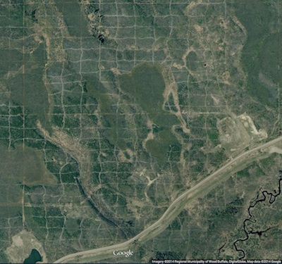
Cutlines for a dense 3D survey at Surmont field, Alberta, Canada. Image: Google Maps.
Cutlines for a dense 3D survey at Surmont field, Alberta, Canada. Image: Google Maps.There are a number of ways to lay out sources and receivers for a 3D seismic survey. In forested areas, a designer may choose a pattern that minimizes the number of trees that need to be felled. Where land access is easier, designers may opt for a pattern that is efficient for the recording crew to deploy and pick up receivers. However, no matter what survey pattern used, most geometries consist of receivers strung together along receiver lines and source points placed along source lines. The pairing of source points with live receiver stations comprises the collection of traces that go into making a seismic volume.
An orthogonal surface pattern, with receiver lines laid out perpendicular to the source lines, is the simplest surface geometry to think about. This pattern can be specified over an area of interest by merely choosing the spacing interval between lines well as the station intervals along the lines. For instance:
xmi = 575000        # Easting of bottom-left corner of grid (m)
ymi = 4710000       # Northing of bottom-left corner (m)
SL = 600            # Source line interval (m)
RL = 600            # Receiver line interval (m)
si = 100            # Source point interval (m)
ri = 100            # Receiver point interval (m)
x = 3000            # x extent of survey (m)
y = 1800            # y extent of survey (m)
We can calculate the number of receiver lines and source lines, as well as the number of receivers and sources for each.
# Calculate the number of receiver and source lines.
rlines = int(y/RL) + 1
slines = int(x/SL) + 1

# Calculate the number of points per line (add 2 to straddle the edges).
rperline = int(x/ri) + 2
sperline = int(y/si) + 2

# Offset the receiver points.
shiftx = -si/2.
shifty = -ri/2.
Computing coordinates
We create a list of x and y coordinates with a nested list comprehension — essentially a compact way to write 'for' loops in Python — that iterates over all the stations along the line, and all the lines in the survey.
# Find x and y coordinates of receivers and sources.
rcvrx = [xmi+rcvr*ri+shifty for line in range(rlines) for rcvr in range(rperline)]
rcvry = [ymi+line*RL+shiftx for line in range(rlines) for rcvr in range(rperline)]

srcx = [xmi+line*SL for line in range(slines) for src in range(sperline)]
srcy = [ymi+src*si for line in range(slines) for src in range(sperline)]
To make a map of the ideal surface locations, we simply pass this list of x and y coordinates to a scatter plot:

Plotting these lists is useful, but it is rather limited by itself. We're probably going to want to do more calculations with these points — midpoints, azimuth distributions, and so on — and put these data on a real map. What we need is to insert these coordinates into a more flexible data structure that can hold additional information.
Shapely, Pandas, and GeoPandas
Shapely is a library for creating and manipulating geometric objects like points, lines, and polygons. For example, Shapely can easily calculate the (x, y) coordinates halfway along a straight line between two points.
Pandas provides high-performance, easy-to-use data structures and data analysis tools, designed to make working with tabular data easy. The two primary data structures of Pandas are:
- Series — a one-dimensional labelled array capable of holding any data type (strings, integers, floating point numbers, lists, objects, etc.)
- DataFrame — a 2-dimensional labelled data structure where the columns can contain many different types of data. This is similar to the NumPy structured array but much easier to use.
GeoPandas combines the capabilities of Shapely and Pandas and greatly simplifies geospatial operations in Python, without the need for a spatial database. GeoDataFrames are a special case of DataFrames that are specifically for representing geospatial data via a geometry column. One awesome thing about GeoDataFrame objects is they have methods for saving data to shapefiles.
So let's make a set of (x,y) pairs for receivers and sources, then make Point objects using Shapely, and in turn add those to GeoDataFrame objects, which we can write out as shapefiles:
# Zip into x,y pairs.
rcvrxy = zip(rcvrx, rcvry)
srcxy = zip(srcx, srcy)

# Create lists of shapely Point objects.
rcvrs = [Point(x,y) for x,y in rcvrxy]
srcs = [Point(x,y) for x,y in srcxy]

# Add lists to GeoPandas GeoDataFrame objects.
receivers = GeoDataFrame({'geometry': rcvrs})
sources = GeoDataFrame({'geometry': srcs})

# Save the GeoDataFrames as shapefiles.
receivers.to_file('receivers.shp')
sources.to_file('sources.shp')
It's a cinch to fire up QGIS and load these files as layers on top of a satellite image or physical topography map. As a survey designer, we can now add, delete, and move source and receiver points based on topography and land issues, sending the data back to Python for further analysis.

All the code used in this post is in an IPython notebook. You can read it, and even execute it yourself. Put your own data in there and see how it comes out!

NEWSFLASH — If you think the geoscientists in your company would like to learn how to play with geological and geophysical models and data — exploring seismic acquisition, or novel well log displays — we can come and get you started! Best of all, we'll help you get up and running on your own data and your own ideas.
If you or your company needs a dose of creative geocomputing, check out our new geocomputing course brochure, and give us a shout if you have any questions. We're now booking for 2015.


 Except where noted, this content is licensed