
Well tie calculus
/ As Matt wrote in March, he is editing a regular Tutorial column in SEG's The Leading Edge. I contributed the June edition, entitled Well-tie calculus. This is a brief synopsis only; if you have any questions about the workflow, or how to get started in Python, get in touch or come to my course.
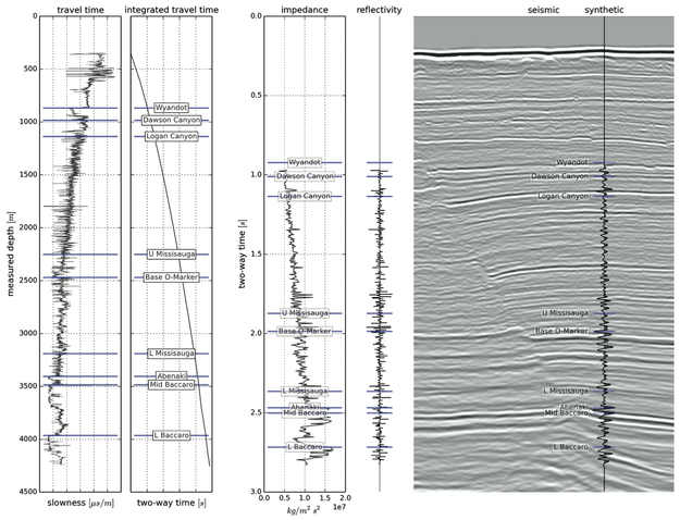
Synthetic seismograms can be created by doing basic calculus on traveltime functions. Integrating slowness (the reciprocal of velocity) yields a time-depth relationship. Differentiating acoustic impedance (velocity times density) yields a reflectivity function along the borehole. In effect, the integral tells us where a rock interface is positioned in the time domain, whereas the derivative tells us how the seismic wavelet will be scaled.
This tutorial starts from nothing more than sonic and density well logs, and some seismic trace data (from the #opendata Penobscot dataset in dGB's awesome Open Seismic Repository). It steps through a simple well-tie workflow, showing every step in an IPython Notebook:
- Loading data with the brilliant LASReader
- Dealing with incomplete, noisy logs
- Computing the time-to-depth relationship
- Computing acoustic impedance and reflection coefficients
- Converting the logs to 2-way travel time
- Creating a Ricker wavelet
- Convolving the reflection coefficients with the wavelet to get a synthetic
- Making an awesome plot, like so...
Final thoughts
If you find yourself stretching or squeezing a time-depth relationship to make synthetic events align better with seismic events, take the time to compute the implied corrections to the well logs. Differentiate the new time-depth curve. How much have the interval velocities changed? Are the rock properties still reasonable? Synthetic seismograms should adhere to the simple laws of calculus — and not imply unphysical versions of the earth.
Matt is looking for tutorial ideas and offers to write them. Here are the author instructions. If you have an idea for something, please drop him a line.


 Except where noted, this content is licensed