All the wedges

Wedges are a staple of the seismic interpreter’s diet. These simple little models show at a glance how two seismic reflections interact with each other when a rock layer thins down to — and below — the resolution limit of the data. We can also easily study how the interaction changes as we vary the wavelet’s properties, especially its frequency content.

Here’s how to make and plot a basic wedge model with Python in the latest version of bruges, v0.4.2:

import bruges as bg
import matplotlib.pyplot as plt

wedge, *_ = bg.models.wedge()

plt.imshow(wedge)

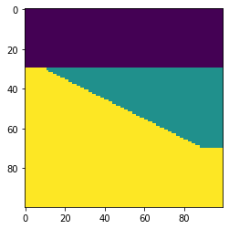
It really is that simple! This model is rather simplistic though: it contains no stratigraphy, and the numerical content of the 2D array is just a bunch of integers. Let’s instead make a P-wave velocity model, with an internal bed of faster rock inside the wedge:

strat = [2.35, (2.40, 2.50, 2.40), 2.65]
wedge, *_ = bg.models.wedge(strat=strat)

plt.imshow(wedge)
plt.colorbar()

We can also choose to make the internal geometry top- or bottom-conformant, mimicking onlap or an unconformity, respectively.

strat = strat=[0, 7*[1,2], 3]
wedge, *_ = bg.models.wedge(strat=strat,
                            conformance='base'
                           )

plt.imshow(wedge)

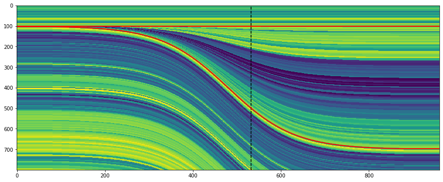
The killer feature of this new function might be using a log to make the stratigraphy, rather than just a few beds. This is straightforward to do with welly, because it makes selecting depth intervals and resampling a bit easier:

import welly

gr = welly.Well.from_las('R-39.las').data['GR']
log_above = gr.to_basis(stop=2620, step=1.0)
log_wedge = gr.to_basis(start=2620, stop=2720, step=1.0)
log_below = gr.to_basis(start=2720, step=1.0)

strat = (log_above, log_wedge, log_below)
depth, width = (100, 400, 100), (40, 200, 40)
wedge, top, base, ref = bg.models.wedge(depth=depth,
                                        width=width,
                                        strat=strat,
                                        thickness=(0, 1.5)
                                       )

plt.figure(figsize=(15, 6))
plt.imshow(wedge, aspect='auto')
plt.axvline(ref, color='k', ls='--')
plt.plot(top, 'r', lw=2)
plt.plot(base, 'r', lw=2)

Notice that the function returns to you the top and base of the wedgy part, as well as the position of the ‘reference’, in this case the well.

I’m not sure if anyone wanted this feature… but you can make clinoform models too:

Lastly, the whole point of all this was to make a synthetic — the forward model of the seismic experiment. We can make a convolutional model with just a few more lines of code:

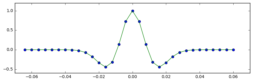
strat = np.array([2.32 * 2.65,  # Layer 1
                  2.35 * 2.60,  # Layer 2
                  2.35 * 2.62,  # Layer 3
                 ])

# Fancy indexing into the rocks with the model.
wedge, top, base, ref = bg.models.wedge(strat=strat)

# Make reflectivity.
rc = (wedge[1:] - wedge[:-1]) / (wedge[1:] + wedge[:-1])

# Get a wavelet.
ricker = bg.filters.ricker(0.064, 0.001, 40)

# Repeated 1D convolution for a synthetic.
syn = np.apply_along_axis(np.convolve, arr=rc, axis=0, v=ricker, mode='same')

That covers most of what the tool can do — for now. I’m working on extending the models to three dimensions, so you will be able to vary layers or rock properties in the 3rd dimension. In the meantime, take these wedges for a spin and see what you can make! Do share your models on Twitter or LinkedIn, and have fun!

What is an Ormsby wavelet anyway?

If you dabble in reflection seismic analysis, you probably know the Ricker wavelet. We’ve visited it a few times on this blog — Evan once showed how to make and plot one, I looked at some analytic properties of it, and we even played golf with it.

The Ricker is everywhere, but it has an important limitation — bandwidth. Its shape in the frequency domain is roughly Gaussian (below, left), which is the reason it only really has one parameter: the central frequency. This kind of spectrum is sometimes okay for older seismic surveys, especially marine data, because it matches the bandwidth reasonably. But for modern surveys, or even old land data, we often want a broader set of frequencies — more of a trapezoidal spectral shape. We need the Ormsby wavelet:

How to make an Ormsby wavelet

The earliest reference I can find to the Ormsby wavelet is in an article by Harold Ryan entitled, Ricker, Ormsby, Klauder, Butterworth — a choice of wavelets, in the September 1994 issue of the CSEG Recorder. It’s not clear at all who Ormsby was, other than “an aeronautical engineer”. And I don’t think anyone outside exploration geophysics knows what an Ormsby is, they just call it a ‘bandpass filter’.

Ryan helpfully provided both a time-domain analytic expression — which turns out to have four typos use the classical definiton of the sinc function — and a plot:

The equation in Ryan, and my modified Figure 3 (right). the result of the equation is in red.

This equation does not produce the wavelet (black) in the plot, however, it produces the one I’ve added in red. If you find this surprising, you shouldn’t — in my experience, it’s very common for the words and/or maths in a paper not to match its figures. [Edit: as noted above, in this case it’s because of how NumPy’s sinc function is defined; see the comment from Robert Kern, below.] We established this at the SEG Repro Zoo in 2018. If an author is not required to produce code or data, it’s not very surprising; and even if they do, the peer review system is not set up for referees to do this kind of check — apart from anything else, it’s far too onerous. But I digress.

After some fiddling around, I realized that the expression being passed to NumPy’s sinc function should be \(ft\), not \(\pi ft\). This produces a result that matches the figure almost exactly (and, counting wiggles, has the right frequency). So here’s the result of that new expression, shown in green here with the original figure (black) and the same red wavelet as above:

This green thing is the wavelet implemented in bruges so it’s easy to produce it; the arguments are the duration (0.4 seconds), the sample interval dt (4 ms) and the corner frequencies f (5, 10, 40, and 45 Hz respectively):

bruges.filters.ormsby(duration=0.4, dt=0.004, f=[5, 10, 40, 45])

What about other examples from the literature?

Good question! Apart from my own Python code in bruges, I did find one or two other implementations:

• A student project from Montclair State University. It produces a similar wavelet, but it’s not quite the same as bruges.

• seismic.jl, the preeminent seismic package for Julia. This matches bruges but then applies a Hamming window.

• GPIAG/SOFI2D software from the Karlsruhe Institute of Technology. This MATLAB/Octave code matches bruges.

• Miong et al. (2007) does not give an implementation, only a plot. I digitized it but can’t quite match it. Have a go!

So it seems from this tiny experiment that only one of the implementations I found matched the figure in the Ryan article perfectly. The other wavelets are variations on the theme. Which is probably fine — after all, they are all only models for real seismic impulses — but in the interests of scientific reproducibility, I think it underscores the importance of transparent methodology and publishing your code.

---

Update on 9 Feb: A conversation in Software Underground revealed that Petrel’s version of the Ormsby wavelet matches the bruges implementation — but with a triangular window multiplied in (similar to how a Hamming window is multiplied into the seismic.jl version.

---

I pushed my Python Jupyter Notebook to the new repro-zoo repository on GitHub. Please feel free to fork this project and add your own attempted reproductions of computational geoscience papers.

The original repro-zoo repo from the 2018 event is on SEG’s GitHub.

---

References

Ryan, H (1994). Ricker, Ormsby, Klauder, Butterworth — a choice of wavelets. CSEG Recorder 19 (7). Available online.

Soo-Kyung Miong, Robert R. Stewart and Joe Wong (2007). Characterizing the near surface with VSP and well logs. CREWES Research Report 19. Available online.

Café con leche

At the weekend, 28 digital geoscientists gathered at MAZ Café in Santa Ana, California, to sprint on some open geophysics software projects. Teams and individuals pushed pull requests — code contributions to open source projects — left, right, and centre. Meanwhile, Senah and her team at MAZ kept us plied with coffee and horchata, with fantastic food on the side.

View fullsize

Because people were helping each other and contributing where they could, I found it a bit hard to stay on top of what everyone was working on. But here are some of the things I heard at the project breakdown on Sunday afternoon:

Gerard Gorman, Navjot Kukreja, Fabio Luporini, Mathias Louboutin, and Philipp Witte, all from the devito project, continued their work to bring Kubernetes cluster management to devito. Trying to balance ease of use and unlimited compute turns out to be A Hard Problem! They also supported the other teams hacking on devito.

Thibaut Astic (UBC) worked on implementing DC resistivity models in devito. He said he enjoyed the expressiveness of devito’s symbolic equation definitions, but that there were some challenges with implementing the grad, div, and curl operator matrices for EM.

Vitor Mickus and Lucas Cavalcante (Campinas) continued their work implementing a CUDA framework for devito. Again, all part of the devito project trying to give scientists easy ways to scale to production-scale datasets.

That wasn’t all for devito. Alongside all these projects, Stephen Alwon worked on adapting segyio to read shot records, Robert Walker worked on poro-elastic models for devito, and Mohammed Yadecuri and Justin Clark (California Resources) contributed too. On the second day, the devito team was joined by Felix Hermann (now Georgia Tech), with Mengmeng Yang, and Ali Siakoohi (both UBC). Clearly there’s something to this technology!

Brendon Hall and Ben Lasscock (Enthought) hacked on an open data portal concept, based on the UCI Machine Learning Repository, coincidentally based just down the road from our location. The team successfully got some examples of open data and code snippets working.

Jesper Dramsch (Heriot-Watt), Matteo Niccoli (MyCarta), Yuriy Ivanov (NTNU) and Adriana Gordon and Volodymyr Vragov (U Calgary), hacked on bruges for the weekend, mostly on its documentation and the example notebooks in the in-bruges project. Yuriy got started on a ray-tracing code for us.

Nathan Jones (California Resources) and Vegard Hagen (NTNU) did some great hacking on an interactive plotting framework for geoscience data, based on Altair. What they did looked really polished and will definitely come in useful at future hackathons.

All in all, an amazing array of projects!

This event was low-key compared to recent hackathons, and I enjoyed the slightly more relaxed atmosphere. The venue was also incredibly supportive, making my life very easy.

A big thank you as always to our sponsors, Dell EMC and Enthought. The presence of the irrepressible David Holmes and Chris Lenzsch (both Dell EMC), and Enthought’s new VP of Energy, Charlie Cosad, was greatly appreciated.

We will definitely be revisiting the sprint concept in the future — einmal ist keinmal, as they say. Devito and bruges both got a boost from the weekend, and I think all the developers did too. So stay tuned for the next edition!

Real and apparent seismic frequency

There's a Jupyter Notebook for you to follow along with this tutorial. You can run it right here in your browser.

---

We often use Ricker wavelets to model seismic, for example when making a synthetic seismogram with which to help tie a well. One simple way to guesstimate the peak or central frequency of the wavelet that will model a particlar seismic section is to count the peaks per unit time in the seismic. But this tends to overestimate the actual frequency because the maximum frequency of a Ricker wavelet is more than the peak frequency. The question is, how much more?

To investigate, let's make a Ricker wavelet and see what it looks like in the time and frequency domains.

>>> T, dt, f = 0.256, 0.001, 25

>>> import bruges
>>> w, t = bruges.filters.ricker(T, dt, f, return_t=True)

>>> import scipy.signal
>>> f_W, W = scipy.signal.welch(w, fs=1/dt, nperseg=256)

When we count the peaks in a section, the assumption is that this apparent frequency — that is, the reciprocal of apparent period or distance between the extrema — tells us the dominant or peak frequency.

To help see why this assumption is wrong, let's compare the Ricker with a signal whose apparent frequency does match its peak frequency: a pure cosine:

>>> c = np.cos(2 * 25 * np.pi * t)
>>> f_C, C = scipy.signal.welch(c, fs=1/dt, nperseg=256)

Notice that the signal is much narrower in bandwidth. If we allowed more oscillations, it would be even narrower. If it lasted forever, it would be a spike in the frequency domain.

Let's overlay the signals to get a picture of the difference in the relative periods:

The practical consequence of this is that if we estimate the peak frequency to be \(f\ \mathrm{Hz}\), then we need to reduce \(f\) by some factor if we want to design a wavelet to match the data. To get this factor, we need to know the apparent period of the Ricker function, as given by the time difference between the two minima.

Let's look at a couple of different ways to find those minima: numerically and analytically.

Find minima numerically

We'll use scipy.optimize.minimize to find a numerical solution. In order to use it, we'll need a slightly different expression for the Ricker function — casting it in terms of a time basis t. We'll also keep f as a variable, rather than hard-coding it in the expression, to give us the flexibility of computing the minima for different values of f.

Here's the equation we're implementing:

$$ w(t, f) = (1 - 2\pi^2 f^2 t^2)\ e^{-\pi^2 f^2 t^2} $$

In Python:

>>> def ricker(t, f):
>>>     return (1 - 2*(np.pi*f*t)**2) * np.exp(-(np.pi*f*t)**2)

Check that the wavelet looks like it did before, by comparing the output of this function when f is 25 with the wavelet w we were using before:

>>> f = 25
>>> np.allclose(w, ricker(t, f=25))
True

Now we call SciPy's minimize function on our ricker function. It itertively searches for a minimum solution, then gives us the x (which is really t in our case) at that minimum:

>>> import scipy.optimize
>>> f = 25
>>> scipy.optimize.minimize(ricker, x0=0, args=(f))

fun: -0.4462603202963996
 hess_inv: array([[1]])
      jac: array([-2.19792128e-07])
  message: 'Optimization terminated successfully.'
     nfev: 30
      nit: 1
     njev: 10
   status: 0
  success: True
        x: array([0.01559393])

So the minimum amplitude, given by fun, is -0.44626 and it occurs at an x (time) of \(\pm 0.01559\ \mathrm{s}\).

In comparison, the minima of the cosine function occur at a time of \(\pm 0.02\ \mathrm{s}\). In other words, the period appears to be \(0.02 - 0.01559 = 0.00441\ \mathrm{s}\) shorter than the pure waveform, which is...

>>> (0.02 - 0.01559) / 0.02
0.22050000000000003

...about 22% shorter. This means that if we naively estimate frequency by counting peaks or zero crossings, we'll tend to overestimate the peak frequency of the wavelet by about 22% — assuming it is approximately Ricker-like; if it isn't we can use the same method to estimate the error for other functions.

This is good to know, but it would be interesting to know if this parameter depends on frequency, and also to have a more precise way to describe it than a decimal. To get at these questions, we need an analytic solution.

Find minima analytically

Python's SymPy package is a bit like Maple — it understands math symbolically. We'll use sympy.solve to find an analytic solution. It turns out that it needs the Ricker function writing in yet another way, using SymPy symbols and expressions for \(\mathrm{e}\) and \(\pi\).

import sympy as sp
t, f = sp.Symbol('t'), sp.Symbol('f')
r = (1 - 2*(sp.pi*f*t)**2) * sp.exp(-(sp.pi*f*t)**2)

Now we can easily find the solutions to the Ricker equation, that is, the times at which the function is equal to zero:

>>> sp.solvers.solve(r, t)
[-sqrt(2)/(2*pi*f), sqrt(2)/(2*pi*f)]

But this is not quite what we want. We need the minima, not the zero-crossings.

Maybe there's a better way to do this, but here's one way. Note that the gradient (slope or derivative) of the Ricker function is zero at the minima, so let's just solve the first time derivative of the Ricker function. That will give us the three times at which the function has a gradient of zero.

>>> dwdt = sp.diff(r, t)
>>> sp.solvers.solve(dwdt, t)
[0, -sqrt(6)/(2*pi*f), sqrt(6)/(2*pi*f)]

In other words, the non-zero minima of the Ricker function are at:

$$ \pm \frac{\sqrt{6}}{2\pi f} $$

Let's just check that this evaluates to the same answer we got from scipy.optimize, which was 0.01559.

>>> np.sqrt(6) / (2 * np.pi * 25)
0.015593936024673521

The solutions agree.

While we're looking at this, we can also compute the analytic solution to the amplitude of the minima, which SciPy calculated as -0.446. We just plug one of the expressions for the minimum time into the expression for r:

>>> r.subs({t: sp.sqrt(6)/(2*sp.pi*f)})
-2*exp(-3/2)

Apparent frequency

So what's the result of all this? What's the correction we need to make?

The minima of the Ricker wavelet are \(\sqrt{6}\ /\ \pi f_\mathrm{actual}\ \mathrm{s}\) apart — this is the apparent period. If we're assuming a pure tone, this period corresponds to an apparent frequency of \(\pi f_\mathrm{actual}\ /\ \sqrt{6}\ \mathrm{Hz}\). For \(f = 25\ \mathrm{Hz}\), this apparent frequency is:

>>> (np.pi * 25) / np.sqrt(6)
32.06374575404661

If we were to try to model the data with a Ricker of 32 Hz, the frequency will be too high. We need to multiply the frequency by a factor of \(\sqrt{6} / \pi\), like so:

>>> 32.064 * np.sqrt(6) / (np.pi)
25.00019823475659

This gives the correct frequency of 25 Hz.

To sum up, rearranging the expression above:

$$ f_\mathrm{actual} = f_\mathrm{apparent} \frac{\sqrt{6}}{\pi} $$

Expressed as a decimal, the factor we were seeking is therefore \(\sqrt{6}\ /\ \pi\):

>>> np.sqrt(6) / np.pi
0.779696801233676

That is, the reduction factor is 22%.

---

Curious coincidence: in the recent Pi Day post, I mentioned the Riemann zeta function of 2 as a way to compute \(\pi\). It evaluates to \((\pi / \sqrt{6})^2\). Is there a million-dollar connection between the humble Ricker wavelet and the Riemann hypothesis?

I doubt it.

Finding Big Bertha with a hot wire

Sunday will be the 131st birthday of General Andrew McNaughton, a Canadian electrical engineer who served in the Canadian Expeditionary Force in the First World War. He was eventually appointed commander of the Canadian Corps Heavy Artillery and went on to serve in the Second World War as well.

So what is a professional soldier doing on a blog about geoscience? Well, McNaughton was part of the revolution of applied acoustics and geophysics that emerged right before and after the First World War.

Along with eminent British physicist Lawrence Bragg, engineer William Sansome Tucker, and physicist Charles Galton Darwin (the other Charles Darwin's grandson), among others, McNaughton applied physics to the big problem of finding the big noisy things that were trying to blow everyone up. They were involved in an arms race of their own — German surveyor Ludger Mintrop was trying to achieve the same goal from the other side of the trenches.

After gaining experience as a gunner, McNaughton became one of a handful of scientists and engineers involved in counter-battery operations. Using novel ranging techniques, these scientists gave the allied forces a substantial advantage over the enemy. Counter-battery fire became an weapon at pivotal battles like Vimy Ridge, and certainly helped expedite the end of the war.

If all this sounds like a marginal way to win a battle, stop think for a second about these artillery. The German howitzer, known as 'Big Bertha' (left), could toss an 820 kg (1800 lb) shell about 12.5 km (7.8 miles). In other words, it was incredibly annoying.

---

Combining technologies

Localization accuracy on the order of 5–10 m on the large majority of gun positions was eventually achieved by the coordinated use of several technologies, including espionage, cartography, aerial reconnaissance photography, and the new counter-measures of flash spotting and sound ranging.

Flash spotting was more or less just what it sounds like: teams of spotters recording the azimuth of artillery flashes, then triangulating artillery positions from multiple observations. The only real trick was in reporting the timing of flashes to help establish that the flashes came from the same gun.

Sound ranging, on the other hand, is a tad more complicated. It seems that Lawrence Bragg was the first to realize that the low frequency sound of artillery fire — which he said lifted him off the privy seat in the outhouse at his lodgings — might be a useful signal. However, microphones were not up to the task of detecting such low frequencies. Furthermore, the signal was masked by the (audible) sonic boom of the shell, as well as the shockwaves of passing shells.

Elsewhere in Belgium, William Tucker had another revelation. Lying inside a shack with holes in its walls, he realized that the 20 Hz pressure wave from the gun created tiny puffs of air through the holes. So he looked for a way to detect this pulse, and came up with a heated platinum wire in a rum jar. The filament's resistance dropped when cooled by the wavefront's arrival through an aperture. The wire was unaffected by the high-frequency shell wave. Later, moving-coil 'microphones' (geophones, essentially) were also used, as well as calibration for wind and temperature. The receivers were coupled with a 5-channel string galvanometer, invented by French engineers, to record traces onto 35-mm film bearing timing marks:

McNaughton continued to develop these technologies through the war, and by the end was successfully locating the large majority of enemy artillery locations, and was even able to specify the calibre of the guns and their probable intended targets. Erster Generalquartiermeister Erich Ludendorff commented at one point in the war: 

“According to a captured English document the English have a well- developed system of sound-ranging which in theory corresponds to our own. Precautions are accordingly to be taken to camouflage the sound: e.g. registration when the wind is contrary, and when there is considerable artillery activity, many batteries firing at the same time, simultaneous firing from false positions, etc.”

---

An acoustic arsenal

The hot-wire artillery detector was not Tucker's only acoustic innovation. He also pioneered the use of acoustic mirrors for aircraft detection. Several of these were built around the UK's east coast, starting around 1915 — the three shown here are at Denge in Kent. They were rendered obselete by the invention of radar around the beginning of World War Two.

Acoustic and seismic devices are still used today in military and security applications, though they are rarely mentioned in applied geophysics textbooks. If you know about any interesting contemporary uses, tell us about it in the comments.

---

According to Crown Copyright terms, the image of McNaughton is out of copyright. The acoustic mirror image is by Paul Russon, licensed CC-BY-SA. The uncredited/unlicensed galvanometer trace is from the excellent Stop, hey, what's that sound article on the geographical imaginations blog; I assume it is out of copyright. The howitzer image is out of copyright.

This post on Target acquisition and counter battery is very informative and has lots of technical details, though most of it pertains to later technology. The Boom! Sounding out the enemy article on ScienceNews for Students is also very nice, with lots of images. 

Easier, better, faster, stronger

Yesterday I pushed a new release of bruges to Python's main package repository, PyPi.  Version 0.3.3 might not sound like an especially auspicious version perhaps, but I'm excited about the new things we've added recently. It has come a long way since we announced it back in 2015, so if you haven't checked it out lately, now's a good time to take another look.

What is bruges again?

Bruges is a...

In other words, nothing fancy — just equations. It is free, open source software. It's aimed at geophysicists who use Python.

How do you install it? The short answer is pip:

    pip install bruges

So what's new?

Here are the highlights of what's been improved and added in the last few months:

• The reflectivity equations in reflection module now work on arrays for the Vp, Vs, and rho values, as well as the theta values. This is about 10 times faster than running a loop over elements; the Zoeppritz solution is 100× faster.
• The various Zoeppritz solutions and the Aki–Richards approximations now return the complex reflectivity and therefore show post-critical amplitudes correctly.
• A new reflection coefficient series function, reflection.reflectivity(), makes it easier to compute offset reflectivities from logs.
• Several new linear and non-linear filters are in bruges.filters, including median (good for seismic horizons), mode (good for waveform classification), symmetric nearest-neighbours or snn, and kuwahara.
• The wavelets ricker(), sweep() (aka Klauder) and ormsby() wavelet now all work for a sequence of frequencies, returning a wavelet bank. Also added a sinc() wavelet, with a taper option to attenuate the sidelobes.
• Added inverse_gardner, and other density and velocity transforms, to petrophysics.
• Added transform.v_rms() (RMS velocity), transform.v_avg() (average velocity) and transform.v_bac() (naïve Backus average). These all operate in a 'cumulative' average-down-to sense.
• Added a coordinate transformation to translate between arbitrarily oriented (x,y) and (inline, line) coordinates.

Want to try using it right now, with no installation? Give it a spin in My Binder! See how easy it is to compute elastic moduli, or offset reflection coefficients, or convert a log to time.  

---

Want to support the development of open source geophysics software? Here's how:

• Use it! This is the main thing we care about.
• Report problems on the project's Issue page.
• Fork the project and make your own changes, then share them back.
• Pay us for the development of functionality you need.

x lines of Python: Let's play golf!

Normally in the x lines of Python series, I'm trying to do something useful in as few lines of code as possible, but — and this is important — without sacrificing clarity. Code golf, on the other hand, tries solely to minimize the number of characters used, and to heck with clarity. This might, and probably will, result in rather obfuscated code.

So today in x lines, we set x = 1 and see what kind of geophysics we can express. Follow along in the accompanying notebook if you like.

A Ricker wavelet

One of the basic building blocks of signal processing and therefore geophysics, the Ricker wavelet is a compact, pulse-like signal, often employed as a source in simulation of seismic and ground-penetrating radar problems. Here's the equation for the Ricker wavelet:

$$ A = (1-2 \pi^2 f^2 t^2) e^{-\pi^2 f^2 t^2} $$

where \(A\) is the amplitude at time \(t\), and \(f\) is the centre frequency of the wavelet. Here's one way to translate this into Python, more or less as expressed on SubSurfWiki:

import numpy as np 
def ricker(length, dt, f):
    """Ricker wavelet at frequency f Hz, length and dt in seconds.
    """
    t = np.arange(-length/2, length/2, dt)
    y = (1.0 - 2.0*(np.pi**2)*(f**2)*(t**2)) * np.exp(-(np.pi**2)*(f**2)*(t**2))
    return t, y

That is alredy pretty terse at 261 characters, but there are lots of obvious ways, and some non-obvious ways, to reduce it. We can get rid of the docstring (the long comment explaining what the function does) for a start. And use the shortest possible variable names. Then we can exploit the redundancy in the repeated appearance of \(\pi^2f^2t^2\)... eventually, we get to:

def r(l,d,f):import numpy as n;t=n.arange(-l/2,l/2,d);k=(n.pi*f*t)**2;return t,(1-2*k)/n.exp(k)

This weighs in at just 95 characters. Not a bad reduction from 261, and it's even not too hard to read. In the notebook accompanying this post, I check its output against the version in our geophysics package bruges, and it's legit:

The 95-character Ricker wavelet in green, with the points computed by the function in BRuges.

What else can we do?

In the notebook for this post, I run through some more algorithms for which I have unit-tested examples in bruges:

• The Ormsby wavelet, reduced from 1545 characters in bruges to 168 characters. (Not bad, considering it took me 111 characters just to express the mathematical equation in the wiki!)
• The 4-term Aki-Richards equation, weighing in at only 179 characters (9.8% of the 1828 characters in bruges).
• The exact Zoeppritz solution for a PP reflection, at 386 characters.

To give you some idea of why we don't normally code like this, here's what the Aki–Richards solution looks like:

def r(a,c,e,b,d,f,t):import numpy as n;w=f-e;x=f+e;y=d+c;p=n.pi*t/180;s=n.sin(p);return w/x-(y/a)**2*w/x*s**2+(b-a)/(b+a)/n.cos((p+n.arcsin(b/a*s))/2)**2-(y/a)**2*(2*(d-c)/y)*s**2

A bit hard to debug! But there is still some point to all this — I've found I've had to really understand Python's order of mathematical operations, and find different ways of doing familiar things. Playing code golf also makes you think differently about repetition and redundancy. All good food for developing the programming brain.

Do have a play with the notebook, which you can even run in Microsoft Azure, right in your browser! Give it a try. (You'll need an account to do this. Create one for free.)

---

Many thanks to Jesper Dramsch and Ari Hartikainen for helping get my head into the right frame of mind for this silliness!

52 Things... Rock Physics

There's a new book in the 52 Things family! 

52 Things You Should Know About Rock Physics is out today, and available for purchase at Amazon.com. It will appear in their European stores in the next day or two, and in Canada... well, soon. If you can't wait for that, you can buy the book immediately direct from the printer by following this link.

The book mines the same vein as the previous volumes. In some ways, it's a volume 2 of the original 52 Things... Geophysics book, just a little bit more quantitative. It features a few of the same authors — Sven Treitel, Brian Russell, Rachel Newrick, Per Avseth, and Rob Simm — but most of the 46 authors are new to the project. Here are some of the first-timers' essays:

• Ludmilla Adam, Why echoes fade.
• Arthur Cheng, How to catch a shear wave.
• Peter Duncan, Mapping fractures.
• Paul Johnson, The astonishing case of non-linear elasticity.
• Chris Liner, Negative Q.
• Chris Skelt, Five questions to ask the petrophysicist.

It's our best collection of essays yet. We're very proud of the authors and the collection they've created. It stretches from childhood stories to linear algebra, and from the microscope to seismic data. There's no technical book like it. 

Supporting Geoscientists Without Borders

Purchasing the book will not only bring you profund insights into rock physics — there's more! Every sale sends $2 to Geoscientists Without Borders, the SEG charity that supports the humanitarian application of geoscience in places that need it. Read more about their important work.

It's been an extra big effort to get this book out. The project was completely derailed in 2015, as we — like everyone else — struggled with some existential questions. But we jumped back into it earlier this year, and Kara (the managing editor, and my wife) worked her magic. She loves working with the authors on proofs and so on, but she doesn't want to see any more equations for a while.

If you choose to buy the book, I hope you enjoy it. If you enjoy it, I hope you share it. If you want to share it with a lot of people, get in touch — we can help. Like the other books, the content is open access — so you are free to share and re-use it as you wish. 

Open source geoscience is _________________

As I wrote yesterday, I was at the Open Source Geoscience workshop at EAGE Vienna 2016 on Monday. Happily, the organizers made time for discussion. However, what passes for discussion in the traditional conference setting is, as I've written before, stilted.

What follows is not an objective account of the proceedings. It's more of a poorly organized collection of soundbites and opinions with no real conclusion... so it's a bit like the actual discussion itself.

TL;DR The main take home of the discussion was that our community does not really know what to do with open source software. We find it difficult to see how we can give stuff away and still make loads of money. 

I'm not giving away my stuff

Paraphrasing a Schlumberger scientist:

Schlumberger sponsors a lot of consortiums, but the consortiums that will deliver closed source software are our favourites.

I suppose this is a way to grab competitive advantage, but of course there are always the other consortium members so it's hardly an exclusive. A cynic might see this position as a sort of reverse advantage — soak up the brightest academics you can find for 3 years, and make sure their work never sees the light of day. If you patent it, you can even make sure no-one else gets to use the ideas for 20 years. You don't even have to use the work! I really hope this is not what is going on.

I loved the quote Sergey Fomel shared; paraphrasing Matthias Schwab, his former advisor at Stanford: 

Never build things you can't take with you.

My feeling is that if a consortium only churns out closed source code, then it's not too far from being a consulting shop. Apart from the cheap labour, cheap resources, and no corporation tax.

Yesterday, in the talks in the main stream, I asked most of the presenters how people in the audience could go and reproduce, or simply use, their work. The only thing that was available was a commerical OpendTect plugin of dGB's, and one free-as-in-beer MATLAB utility. Everything else was unavailble for any kind of inspection, and in one case the individual would not even reveal the technology framework they were using.

Support and maintenance

Paraphrasing a Saudi Aramco scientist:

There are too many bugs in open source, and no support. 

The first point is, I think, a fallacy. It's like saying that Wikipedia contains inaccuracies. I'd suggest that open source code has about the same number of bugs as proprietary software. Software has bugs. Some people think open source is less buggy; as Linus Torvalds said: "Given enough eyeballs, all bugs are shallow." Kristofer Tingdahl (dGB) pointed out that the perceived lack of support is a business opportunity for open source community. Another participant mentioned the importance of having really good documentation. That costs money of course, which means finding ways for industry to support open source software development.

The same person also said something like:

[Open source software] changes too quickly, with new versions all the time.

...which says a lot about the state of application management in many corporations and, again, may represent opportunity rather than a threat to open source movement.

Only in this industry (OK, maybe a couple of others) will you hear the impassioned cry, "Less change!" 

The fog of torpor

When a community is falling over itself to invent new ways to do things, create new value for people, and find new ways to get paid, few question the sharing and re-use of information. And by 'information' I mean code and data, not a few PowerPoint slides. Certainly not all information, but lots. I don't know which is the cause and which is the effect, but the correlation is there.

In a community where invention is slow, on the other hand, people are forced to be more circumspect, and what follows is a cynical suspicion of the motives of others. Here's my impression of the dynamic in the room during the discussion on Monday, and of course I'm generalizing horribly:

• Operators won't say what they think in front of their competitors
• Vendors won't say what they think in front of their customers and competitors
• Academics won't say what they think in front of their consortium customers sponsors
• Students won't say what they think in front of their advisors and potential employers

This all makes discussion a bit stilted. But it's not impossible to have group discussions in spite of these problems. I think we achieved a real, honest conversation in the two Unsessions we're done in Calgary, and I think the model we used would work perfectly in all manner of non-technical and in technical settings. We just have to start doing it. Why our convention organizers feel unable to try new things at conferences is beyond me.

I can't resist finishing on something a person at Chevron said at the workshop:

I'm from Chevron. I was going to say something earlier, but I thought maybe I shouldn't.

This just sums our industry up.

Open source FWI, I mean geoscience

I'm being a little cheeky. Yesterday's Open Source Geoscience workshop at EAGE was not really only about full waveform inversion (FWI). True, it was mostly about geophysics, but there was quite a bit of new stuff too.

But there was quite a bit on FWI.

The session echoed previous EAGE sessions on the same subject in 2006 and 2012, and was chaired by Filippo Broggini (of ETH Zürich), Sergey Fomel (University of Texas), Thomas Günther (LIAG Hannover), and Russell Hewett (Total, unfortunately not present). It started with a look at core projects like Madagascar and OpendTect. There were some (for me) pretty hard core, mathematics-heavy contributions. And we got a tour of some new and newish projects that are seeking users and/or contributors. Rather than attempting to cover everything, I'm going to exercise my (biased and ill-gotten) judgment and focus on some highlights from the day.

Filippo Broggini started by reminding us of why Joe Dellinger (BP) started this recurrent workshop a decade ago. Here's how Joe framed the value of open source to our community:

The economic benefits of a collaborative open-source exploration and production processing and research software environment would be enormous. Skilled geophysicists could spend more of their time doing innovative geophysics instead of mediocre computer science. Technical advances could be quickly shared and reproduced instead of laboriously re-invented and reverse-engineered. Oil companies, contractors, academics, and individuals would all benefit.

Did I mention that he wrote that 10 years ago?

Lessons learned from the core projects

Kristofer Tingdahl (dGB) then gave the view from his role as CEO of dGB Earth Sciences, the company behind OpendTect, the free and open source geoscience interpretation tool. He did a great job of balancing the good (their thousands of users, and their SEG Distinguished Achievement Award 2016) with the less good (the difficulty of building a developer community, and the struggle to get beyond only hundreds of paying users). His great optimism and natural business instinct filled us all with hope.

The irrepressible Sergey Fomel summed up 10 years of Madagascar's rise. In the journey from v0.9 to v2.0, the projects has moved from SourceForge to GitHub, gone from 6 to 72 developers, jumped from 30 to 260 reproducible papers, and been downloaded over 40 000 times. He also shared the story of his graduate experience at Stanford, where he was involved in building the first 'reproducible science' system with Jon Claerbout in the early 1990s. Un/fortunately, it turned out to be unreproducible, so he had to build Madagascar.

It's not (yet?) a core project, but John Stockwell (Colorado School of Mines) talked about OpenSeaSeis and barely mentioned SeismicUnix. This excellent little seismic processing project is now owned by CSM, after its creator, Bjoern Olofsson, had to give it up when he went to work for a corporation (makes sense, right? o_O ). The tool includes SeaView, a standalone SEGY viewer, as well as a graphical processing flow composer called XSeaSeis. IT prides itself on its uber-simple architecture (below). Want a gain step? Write gain.so and you're done. Perfect for beginners.

Jeffrey Shragge (UWA), Bob Clapp (SEP), and Bill Symes (Rice) provided some perspective from groups solving big math problems with big computers. Jeff talked about coaxing Madgascar — or M8R as the cool kids apparently refer to it — into the cloud, where it can chomp through 100 million core hours without setting tings on fire. This is a way for small enterprises and small (underfunded) research teams to get big things done. Bob told us about a nifty-looking HTML5 viewer for subsurface data... which I can't find anywhere. And Bill talked about 'mathematical fidelty'. and its application to solving large, expensive problems without creating a lot of intermediate data. His message: the mathematics should provide the API.

New open source tools in geoscience

The standout of the afternoon for me was University of Vienna post-doc Eun Young Lee's talk about BasinVis. The only MATLAB code we saw — so not truly open source, though it might be adapted to GNU Octave — and the only strictly geological package of the day. To support her research, Eun Young has built a MATLAB application for basin analysis, complete with a GUI and some nice visuals. This one shows a geological surface, gridded in the tool, with a thickness map projected onto the 'floor' of the scene:

I'm poorly equipped to write much about the other projects we heard about. For the record and to save you a click, here's the list [with notes] from my 'look ahead' post:

• SES3D [presented by Alexey Gokhberg], a package from ETHZ for seismic modeling and inversion.
• OpenFOAM [Gérald Debenest], a new open source toolbox for fluid mechanics.
• PyGIMLi [Carsten Rücker], a geophysical modeling and inversion package.
• PySIT [Laurent Demanet], the Python seismic imaging toolbox that Russell Hewett started while at MIT.
• Seismic.jl [Nasser Kazemi] and jInv [Eldad Haber], two [modeling and inversion] Julia packages.

My perception is that there is a substantial amount of overlap between all of these packages except OpenFOAM. If you're into FWI you're spoilt for choice. Several of these projects are at the heart of industry consortiums, so it's a way for corporations to sponsor open source projects, which is awesome. However, most of them said they have closed-source components which only the consortium members get access to, so clearly the messaging around open source — the point being to accelerate innovation, reduce bugs, and increase value for everyone — is missing somewhere. There's still this idea that secrecy begets advantage begets profit, but this idea is wrong. Hopefully the other stuff, which may or may not be awesome, gets out eventually.

---

I gave a talk at the end of the day, about ways I think we can get better at this 'openness' thing, whatever it is. I will write about that some time soon, but in the meantime you're welcome to see my slides here.

Finally, a little time — two half-hour slots — was set aside for discussion. I'll have a go at summing that up in another post. Stay tuned!

BasinVis image © 2016 Eun Young Lee, used with permission. OpenSeaSeis image © 2016 Center for Wave Phenomena