It goes in the bin

The cells of a digital image sensor. CC-BY-SA Natural Philo.

Inlines and crosslines of a 3D seismic volume are like the rows and columns of the cells in your digital camera's image sensor. Seismic bins are directly analogous to pixels — tile-like containers for digital information. The smaller the tiles, the higher the maximum realisable spatial resolution. A square survey with 4 million bins (or 4 megapixels) gives us 2000 inlines and 2000 crosslines to interpret, after processing the data of course. Small bins can mean high resolution, but just as with cameras, bin size is only one aspect of image quality.

Unlike your digital camera however, seismic surveys don't come with a preset number of megapixels. There aren't any bins until you form them. They are an abstraction.

Making bins

This post picks up where Laying out a seismic survey left off. Follow the link to refresh your memory; I'll wait here. 

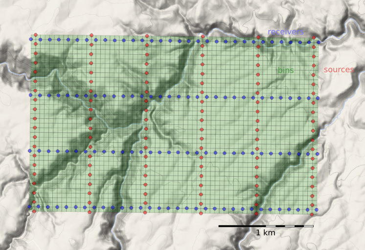
At the end of that post, we had a network of sources and receivers, and the Notebook showed how I computed the midpoints of the source–receiver pairs. At the end, we had a plot of the midpoints. Next we'd like to collect those midpoints into bins. We'll use the so-called natural bins of this orthogonal survey — squares with sides half the source and receiver spacing.

Just as we represented the midpoints as a GeoSeries of Point objects, we will represent  the bins with a GeoSeries of Polygons. GeoPandas provides the GeoSeries; Shapely provides the geometries; take a look at the IPython Notebook for the code. This green mesh is the result, and will hold the stacked traces after processing.

Fetching the traces within each bin

To create a CMP gather like the one we modelled at the start, we need to grab all the traces that have midpoints within a particular bin. And we'll want to create gathers for every bin, so it is a huge number of comparisons to make, even for a small example such as this: 128 receivers and 120 sources make 15 320 midpoints. In a purely GIS environment, we could perform a spatial join operation between the midpoint and bin GeoDataFrames, but instead we can use Shapely's contains method inside nested loops. Because of the loops, this code block takes a long time to run.

# Make a copy because I'm going to drop points as I
# assign them to polys, to speed up subsequent search.
midpts = midpoints.copy()

offsets, azimuths = [], [] # To hold complete list.

# Loop over bin polygons with index i.
for i, bin_i in bins.iterrows():
    
    o, a = [], [] # To hold list for this bin only.
    
    # Now loop over all midpoints with index j.
    for j, midpt_j in midpts.iterrows():
        if bin_i.geometry.contains(midpt_j.geometry):
            # Then it's a hit! Add it to the lists,
            # and drop it so we have less hunting.
            o.append(midpt_j.offset)
            a.append(midpt_j.azimuth)
            midpts = midpts.drop([j])
            
    # Add the bin_i lists to the master list
    # and go around the outer loop again.
    offsets.append(o)
    azimuths.append(a)
    
# Add everything to the dataframe.    
bins['offsets'] = gpd.GeoSeries(offsets)
bins['azimuths'] = gpd.GeoSeries(azimuths)

After we've assigned traces to their respective bins, we can make displays of the bin statistics. Three common views we can look at are:

1. A spider plot to illustrate the offset and azimuth distribution.
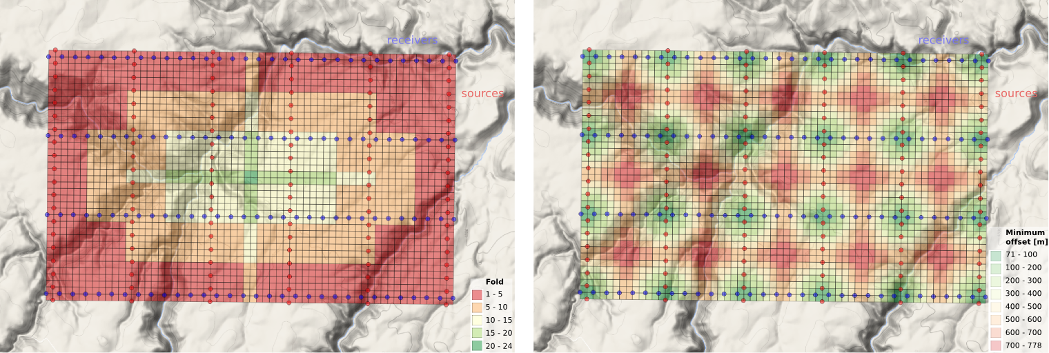
2. A heat map of the number of traces contributing to each bin, usually called fold.
3. A heat map of the minimum offset that is servicing each bin. 

The spider plot is easily achieved with Matplotlib's quiver plot:

And the arrays representing our data are also quite easy to display as heatmaps of fold (left) and minimum offset (right): 

In the next and final post of this seismic survey mini-series, we'll analyze the impact of data quality when there are gaps and shifts in the source and receiver stations from these idealized locations.

Last thought: if the bins of a seismic survey are like a digital camera's image sensor, then what is the apparatus that acts like a lens?