The open subsurface stack

Two observations:

1. Agile has been writing about open source software for geology and geophysics for several years now (for example here in 2011 and here in 2016). Progress is slow. There are lots of useful tools, but lots of gaps too. Some new tools have appeared, others have died. Conclusion: a robust and trusted open stack is not going to magically appear.

2. People — some of them representing large corporations — are talking more than ever about industry collaboration. Open data platofrms are appearing all over the place. And several times at the DigEx conference in Oslo last week I heard people talk about open source and open APIs. Some organizations, notably Equinor, seem to really mean business. Conclusion: there seems to be a renewed appetite for open source subsurface software.

A quick reminder of what ‘open’ means; paraphrasing The Open Definition and The Open Source Definition in a sentence:

“Open data, content and code can be freely used, modified, and shared by anyone for any purpose.”

The word ‘open’ is being punted around quite a bit recently, but you have to read the small print in our business. Just as OpenWorks is not ‘open’ by the definition above, neither is OpenSpirit (remember that?), nor the Open Earth Community. (I’m not trying to pick on Halliburton but the company does seem drawn to the word, despite clearly not quite understanding it.)

The conditions are perfect

Earlier I said that a robust and trusted ‘stack’ (a collection of software that, ideally, does all the things we need) is not going to magically appear. What do I mean by ‘robust and trusted’? It goes far beyond ‘just code’ — writing code is the easy bit. It means thoroughly tested, carefully documented, supported, and maintained. All that stuff takes work, and work takes people and time. And people and time mean money.

Two more observations:

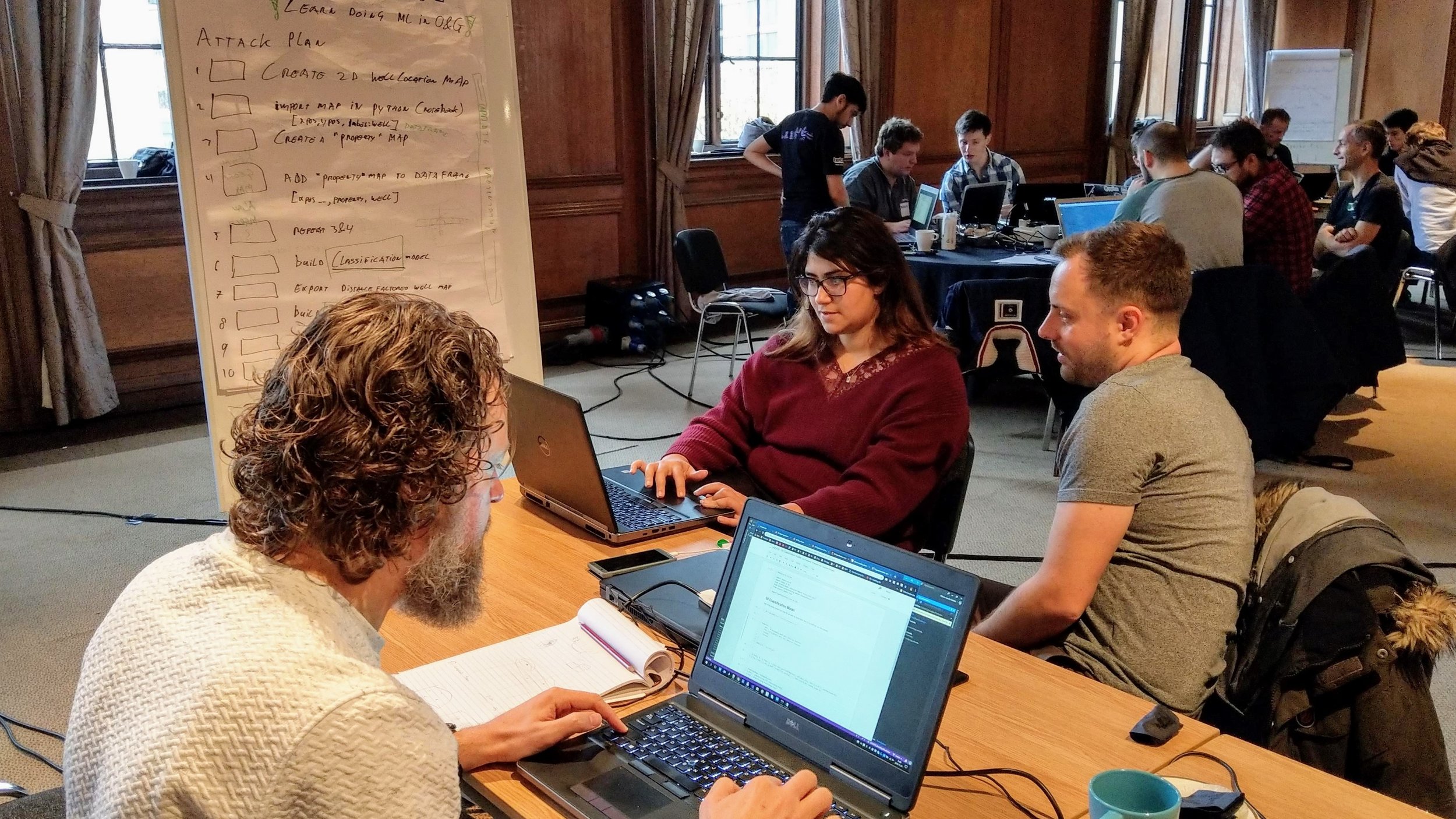
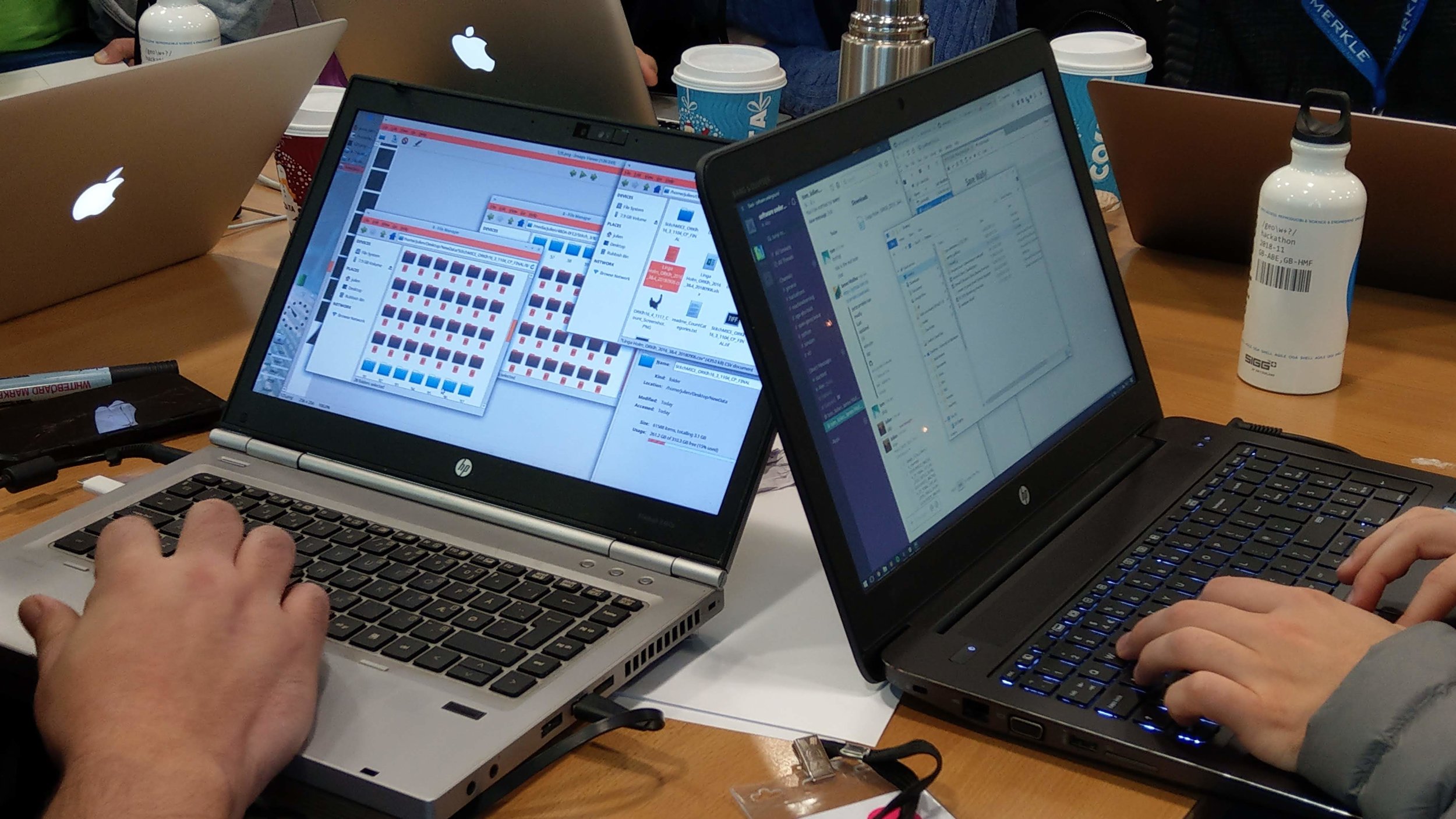
1. Agile has been teaching geocomputing like crazy — 377 people in the last year. In our class, the participants install a lot of Python libraries, including a few from the open subsurface stack: segyio, lasio, welly, and bruges. Conclusion: a proto-stack exists already, hundreds of users exist already, and some training and support exist already.

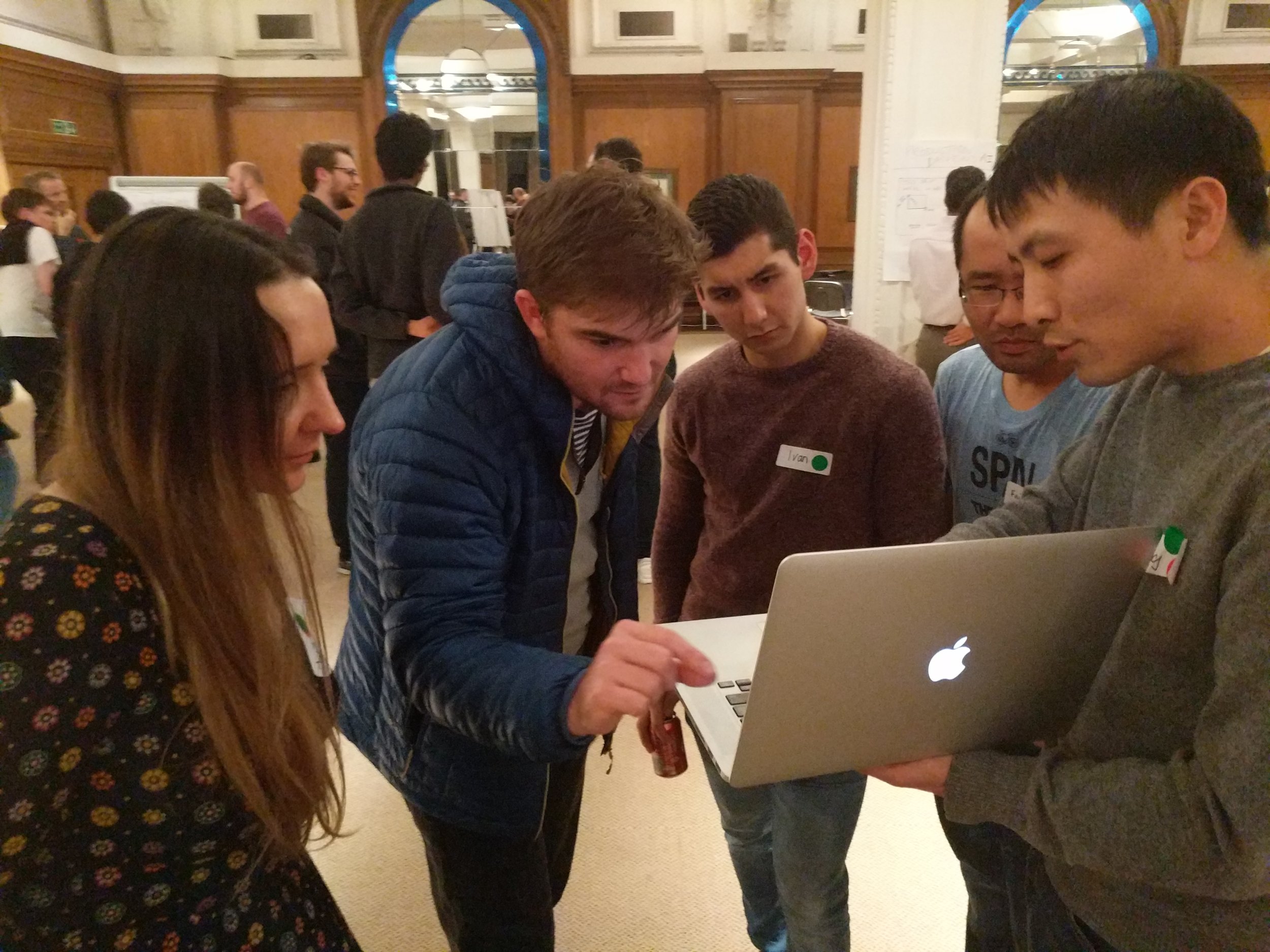
2. The Software Underground has over 1200 members (you should sign up, it’s free!). That’s a lot of people that care passionately about computers and rocks. The Python and machine learning communies are especially active. Conclusion: we have a community of talented scientists and developers that want to get good science done.

So what’s missing? What’s stopping us from taking open source subsurface tech to the next level?

Nothing!

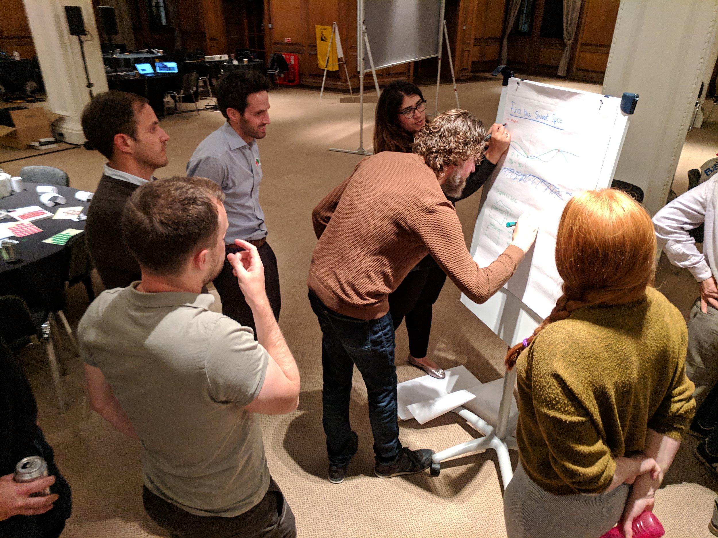
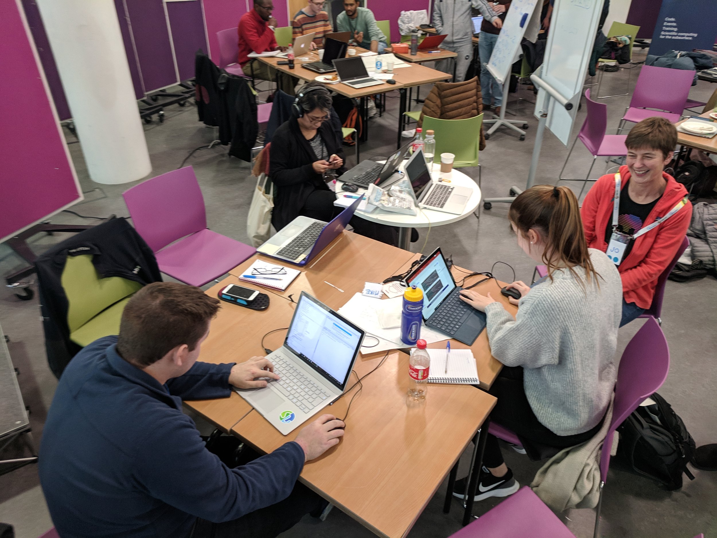
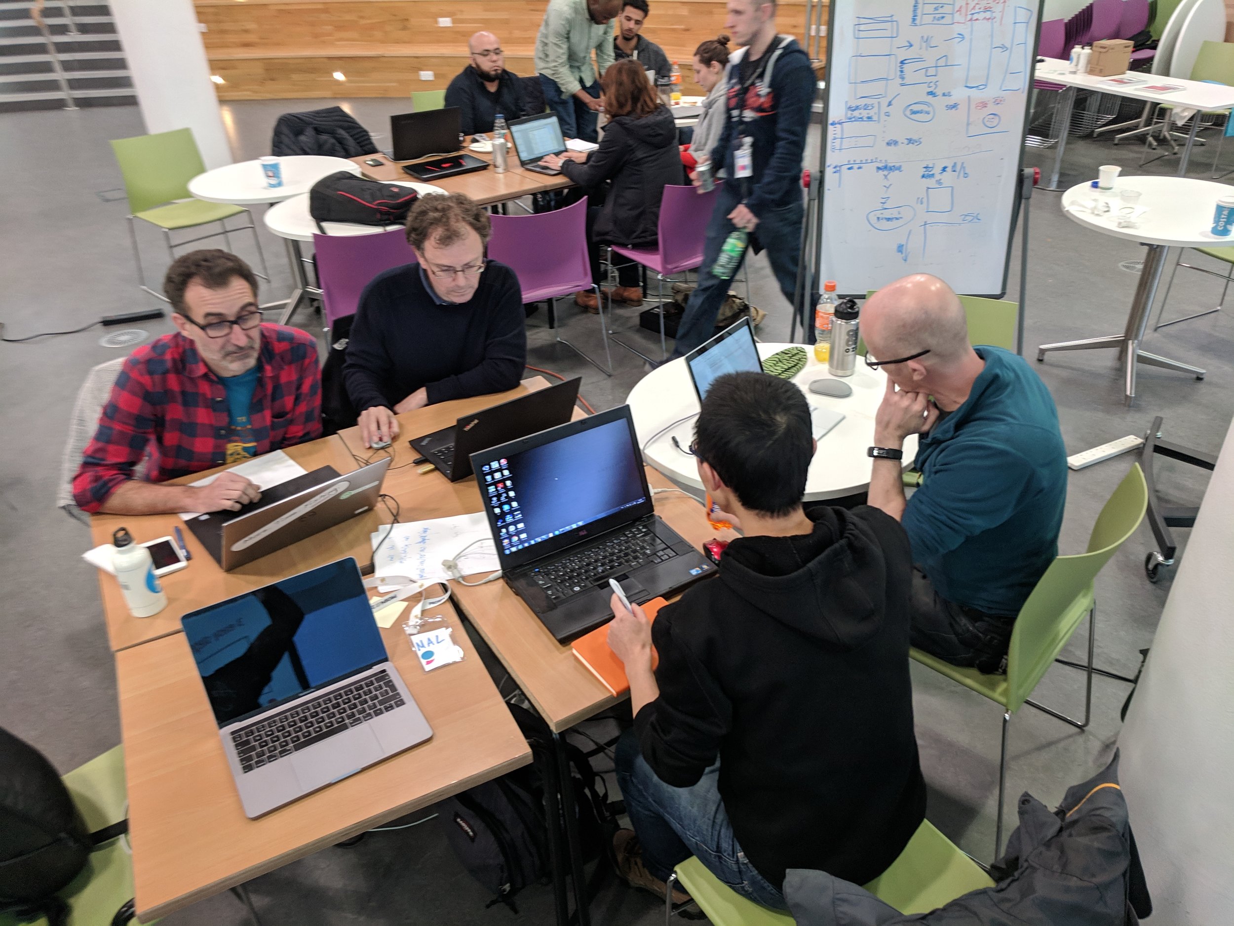
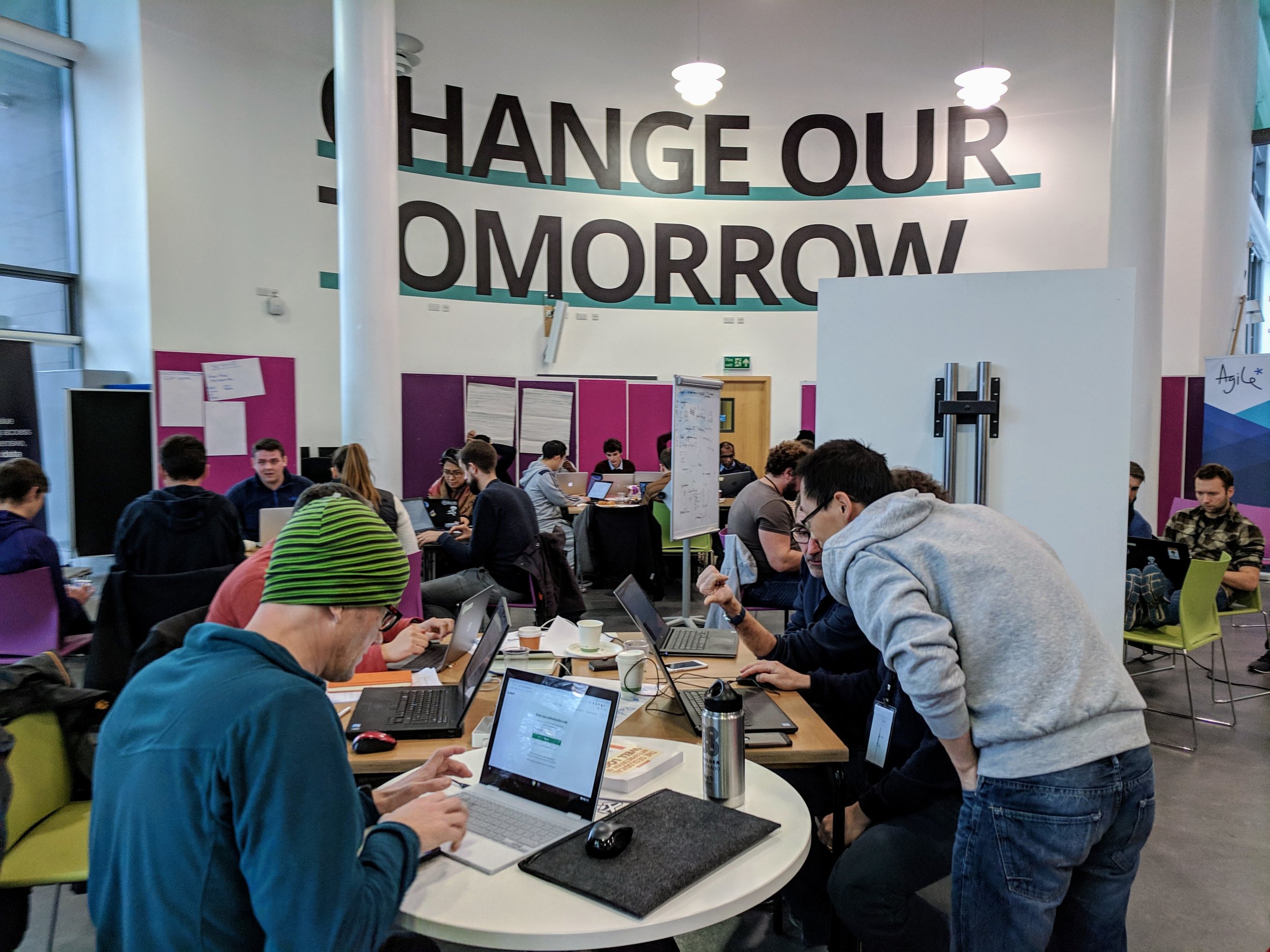
Nothing is stopping us. And I’ve reached the conclusion that we need to provide care and feeding to this proto-stack, and this needs to start now. This is what the TRANSFORM 2019 unconference is going to be about. About 40 of us (you’re invited!) will spend five days working on some key questions:

• What libraries are in the Python ‘proto-stack’? What kind of licenses do they have? Who are the maintainers?

• Do we need a core library for the stack? Something to manage some basic data structures, units of measure, etc.

• What are we calling it, who cares about it, and how are we going to work together?

• Who has the capacity to provide attention, developer time, existing code, or funds to the stack?

• Where are the gaps in the stack, and which ones need to be filled first?

We won’t finish all this at the unconference. But we’ll get started. We’ll produce a lot of ideas, plans, roadmaps, GitHub issues, and new code. If that sounds like fun to you, and you can contribute something to this work — please come. We need you there! Get more info and sign up here.

---

Read the follow-up post >>> What’s happening at TRANSFORM?

---

Thumbnail photo of the Old Man of Hoy by Tom Bastin, CC-BY on Flickr.

What is the fastest axis of an array?

One of the participants in our geocomputing course asked us a tricky question earlier this year. She was a C++ and Java programmer — we often teach experienced programmers who want to learn about Python and/or machine learning — and she worked mostly with seismic data. She had a question related to the performance of n-dimensional arrays: what is the fastest axis of a NumPy array?

I’ve written before about how computational geoscience is not ‘software engineering’ and not ‘computer science’, but something else. And there’s a well established principle in programming, first expressed by Michael Jackson:

“We follow two rules in the matter of optimization:
Rule 1: Don’t do it.
Rule 2 (for experts only). Don’t do it yet — that is, not until you have a perfectly clear and unoptimized solution.”

Most of the time the computer is much faster than we need it to be, so we don’t spend too much time thinking about making our programs faster. We’re mostly concerned with making them work, then making them correct. But sometimes we have to think about speed. And sometimes that means writing smarter code. (Other times it means buying another GPU.) If your computer spends its days looping over seismic volumes extracting slices for processing, you should probably know whether you want to put time in the first dimension or the last dimension of your array.

The 2D case

Let’s think about a two-dimensional case first — imagine a small 2D array, also known as a matrix in some contexts. I’ve coloured in the elements of the matrix to make the next bit easier to understand.

When we store a matrix in a computer (or an image, or any array), we have a decision to make. In simple terms, the computer’s memory is like a long row of boxes, each with a unique address — shown here as a 3-digit hexadecimal number:

We can only store one number in each box, so we’re going to have to flatten the 2D array. The question is, do we put the rows in together, effectively splitting up the columns, or do we put the columns in together? These two options are commonly known as ‘row major’, or C-style, and ‘column major’, or Fortran-style:

Let’s see what this looks like in terms of the indices of the elements. We can plot the index number on each axis vs. the position of the element in memory. Notice that the C-ordered elements are contiguous in axis 0:

View fullsize

If you spend a lot of time loading seismic data, you probably recognize this issue — it’s analgous to how traces are stored in a SEG-Y file. Of couse, with seismic data, two dimensions aren’t always enough…

Higher dimensions

The problem multiplies at higher dimensions. If we have a cube of data, then C-style ordering results in the first dimension having large contiguous chunks, and the last dimension being broken up. The middle dimension is somewhere in between. As before, we can illustrating this by plotting the indices of the data. This time I’m highlighting the positions of the elements with index 2 (i.e. the third element) in each dimension:

So if this was a seismic volume, we might organize inlines in the first dimension, and travel-time in the last dimension. That way, we can access inlines very quickly, but timeslices will take longer.

In Fortran order, which we can optionally specify in NumPy, the situation is reversed. Now the fast axis is the last axis:

Lots of programming languages and libraries use row-major memory layout, including C, C++, Torch and NumPy. Most others use column-major ordering, including MATLAB, R, Julia, and Fortran. (Some other languages, such as Java and .NET, use a variant of row-major order called Iliffe vectors). NumPy calls row-major order ‘C’ (for C, not for column), and column-major ‘F’ for Fortran (thankfully they didn’t use R, for R not for row).

I expect it’s related to their heritage, but the Fortran-style languages also start counting at 1, whereas the C-style languages, including Python, start at 0.

What difference does it make?

The main practical difference is in the time it takes to access elements in different orientations. It’s faster for the computer to take a contiguous chunk of neighbours from the memory ‘boxes’ than it is to have to ‘stride’ across the memory taking elements from here and there.

How much faster? To find out, I made datasets full of random numbers, then selected slices and added 1 to them. This was the simplest operation I could think of that actually forces NumPy to do something with the data. Here are some statistics — the absolute times are pretty irrelevant as the data volumes I used are all different sizes, and the speeds will vary on different machines and architectures:

• 2D data: 3.6× faster. Axis 0: 24.4 µs, axis 1: 88.1 µs (times relative to first axis: 1, 3.6).

• 3D data: 43× faster. 229 µs, 714 µs, 9750 µs (relatively 1, 3.1, 43).

• 4D data: 24× faster. 1.27 ms, 1.36 ms, 4.77 ms, 30 ms (relatively 1, 1.07, 3.75, 23.6).

• 5D data: 20× faster. 3.02 ms, 3.07 ms, 5.42 ms, 11.1 ms, 61.3 ms (relatively 1, 1.02, 1.79, 3.67, 20.3).

• 6D data: 5.5× faster. 24.4 ms, 23.9 ms, 24.1 ms, 37.8 ms, 55.3 ms, 136 ms (relatively 1, 0.98, 0.99, 1.55, 2.27, 5.57).

These figures are more or less simply reversed for Fortran-ordered arrays (see the notebook for datails).

Clearly, the biggest difference is with 3D data, so if you are manipulating seismic data a lot and need to access the data in that last dimension, usually travel-time, you might want to think about ways to reduce this overhead.

What difference does it really make?

The good news is that, for most of us most of the time, we don’t have to worry about any of this. For one thing, NumPy’s internal workings (in particular, its universal functions, or ufuncs) know which directions are fastest and take advantage of this when possible. For another thing, we generally try to avoid looping over arrays at all, leaving the iterative components of our algorithms to the ufuncs — so the slicing speed isn’t a factor. Even when it is a factor, or if we can’t avoid looping, it’s often not the bottleneck in the code. Usually the guts of our algorithm are what are slowing the computer down, not the access to memory. The net result of all this is that we don’t often have to think about the memory layout of our arrays.

So when does it matter? The following situations merit a bit of thought:

• When you’re doing a very large number of accesses to memory or disk. Saving a few microseconds might add up to a lot if you’re doing it a billion times.

• When the objects you’re accessing are very large. Reading and writing elements of a 200GB array in memory brings new challenges compared to handling a few gigabytes.

• Reading and writing data files — really just another kind of memory — brings all the same issues. Reading a chunk of contiguous data is much faster than reading bytes from here and there. Landmark’s BRI seismic data format, Schlumberger’s ZGY files, and HDF5 files, all implement strategies to help make reading arbitrary data faster.

• Converting code from other languages, especially MATLAB, although do realize that other languages may have their own indexing rules, as well as differing in how they store n-dimensional arrays.

If you determine that you do need to think about this stuff, then you’re going to need to read this essay about NumPy’s internal representations, and I recommend checking out this blog post by Eli Bendersky too.

There you have it. Very occasionally we scientists also need to think a bit about how computers work… but most of the time someone has done that thinking for us.

Some of the figures and all of the timings for this post came from this notebook — please have a look. If you have anything to add, or (better yet) correct, please get in touch. I’d love to hear from you.

2018 retrospective

It’s almost the end of another trip around the sun. I hope it’s been kind to you. I mean, I know it’s sometimes hard to see the kindness for all the nonsense and nefariousness in <ahem> certain parts of the world, but I hope 2018 at least didn’t poke its finger in your eye, or set fire to any of your belongings. If it did — may 2019 bring you some eye drops and a fire extinguisher.

Anyway, at this time of year, I like to take a quick look over my shoulder at the past 12 months. Since I’m the over-sharing type, I like to write down what I see and put it on the Internet. I apologize, and/or you’re welcome.

Top of the posts

We’ve been busier than ever this year, and the blog has taken a bit of a hit. In spite of the reduced activity (only 45 posts, compared to 53 last year), traffic continues to grow and currently averages 9000 unique visitors per month. These were the most visited posts in 2018:

• Big open data, or is it? — about the amazing Volve dataset released by Equinor earlier this year. Don’t miss the follow-up post about its licensing: Volve: not open after all, in which I discuss the license that Equinor chose.

• x lines of Python: contour maps — making nice contour maps in Python (strictly a 2017 post, but almost all of its traffic came in 2018).

• What is scientific computing? — the emergence of the ‘digital geoscientist’.

• Results from the AAPG machine learning unsession — what happened in Salt Lake City.

• Jounce, crackle and pop — derivatives of displacement you never knew you cared about.

Last December’s post, No more rainbows, got more traffic this year than any of these posts. And, yet again, k is for wavenumber got more than any. What is it with that post??

Where in the world?

Every year I take a look at where our people are reading the blog from (according to Google). We’ve travelled more than usual this year too, so I’ve added our various destinations to the map… it makes me realize we’re still missing most of you.

1. Houston (number 1 last year)

2. London (up from 3)

3. Calgary (down from 2)

4. Stavanger (6)

5. Paris (9)

6. New York (—)

7. Perth (4)

8. Bangalore (—)

9. Jakarta (—)

10. Kuala Lumpur (8)

Together these cities capture at least 15% of our readship. New York might be an anomaly related to the location of cloud infrastructure there. (Boardman, Oregon, shows up for the same reason.) But who knows what any of these numbers mean…

Work

People often ask us how we earn a living, and sometime I wonder myself. But not this year: there was a clear role for us to play in 2018 — training the next wave of digital scientists and engineers in subsurface.

• We continued the machine learning project on GPR interpretation that we started last year.

• We revived Pick This and have it running on a private corporate cloud at a major oil company, as well as on the Internet.

• We have spent 63 days in the classroom this year, and taught 325 geoscientists the fundamentals of Python and machine learning.

• Apart from the 6 events of our own that we organized, we were involved in 3 other public hackathons and 2 in-house hackathons.

• We hired awesome digital geologist Robert Leckenby (right) full time. 

The large number of people we’re training at the moment is especially exciting, because of what it means for the community. We spent 18 days in the classroom and trained 139 scientists in the previous four years combined — so it’s clear that digital geoscience is important to people today. I cannot wait to see what these new coders do in 2019 and beyond!

The hackathon trend is similar: we hosted 310 scientists and engineers this year, compared to 183 in the four years from 2013 to 2017. Numbers are only numbers of course, but the reality is that we’re seeing more mature projects, and more capable coders, at every event. I know it’s corny to say so, but I feel so lucky to be a scientist today, there is just so much to do.

Cheers to you

Agile is, as they say, only wee. And we all live in far-flung places. But the Intertubes are a marvellous thing, and every week we meet new people and have new conversations via this blog, and on Twitter, and the Software Underground. We love our community, and are grateful to be part of it. So thank you for seeking us out, cheering us on, hiring us, and just generally being a good sport about things.

From all of us at Agile, have a fantastic festive season — and may the new year bring you peace and happiness.

The London hackathon

At the end of November I reported on the projects at the Oil & Gas Authority’s machine learning hackathon in Aberdeen. This post is about the follow-up event at London Olympia.

---

Like the Aberdeen hackathon the previous weekend, the theme was ‘machine learning’. The event unfolded in the Apex Room at Olympia, during the weekend before the PETEX conference. The venue was excellent, with attentive staff and top-notch catering. Thank you to the PESGB for organizing that side of things.

Thirty-eight digital geoscientists spent the weekend with us, and most of them also took advantage of the bootcamp on Friday; at least a dozen of those had not coded at all before the event. It’s such a privilege to work with people on their skills at these events, and to see them writing their own code over the weekend.

Here’s the full list of projects from the event…

---

Sweet spot hunting

Sweet Spot Sweat Shop: Alan Wilson, Geoff Chambers, Marco van der Linden, Maxim Kotenev, Rowan Haddad.

Project: We’ve seen a few people tackling the issue of making decisions from large numbers of realizations recently. The approach here was to generate maps of various outputs from dynamic modeling and present these to the user in an interactive way. The team also had maps of sweet spots, as determined by simulation, and they attempted to train models to predict these sweetspots directly from the property maps. The result was a unique and interesting exploration of the potential for machine learning to augment standard workflows in reservoir modeling and simulation. Project page. GitHub repo.

---

An intelligent dashboard

Dash AI: Vincent Penasse, Pierre Guilpain.

Project: Vincent and Pierre believed so strongly in their project that they ran with it as a pair. They started with labelled production history from 8 wells in a Pandas dataframe. They trained some models, including decision trees and KNN classifiers, to recognizedata issues and recommend required actions. Using skills they gained in the bootcamp, they put a flask web app in front of these to allow some interaction. The result was the start of an intelligent dashboard that not only flagged issues, but also recommended a response. Project page.

This project won recognition for impact.

---

Predicting logs ahead of the bit

Team Mystic Bit: Connor Tann, Lawrie Cowliff, Justin Boylan-Toomey, Patrick Davies, Alessandro Christofori, Dan Austin, Jeremy Fortun.

Project: Thinking of this awesome demo, I threw down the gauntlet of real-time look-ahead prediction on the Friday evening, and Connor and the Mystic Bit team picked it up. They did a great job, training a series of models to predict a most likely log (see right) as well as upper and lower bounds. In the figure, the bit is currently at 1770 m. The model is shown the points above this. The orange crosses are the P90, P50 and P10 predictions up to 40 m ahead of the bit. The blue points below 1770 m have not yet been encountered. Project page. GitHub repo.

This project won recognition for best execution.

---

The seals make a comeback

Selkie Se7en: Georgina Malas, Matthew Gelsthorpe, Caroline White, Karen Guldbaek Schmidt, Jalil Nasseri, Joshua Fernandes, Max Coussens, Samuel Eckford.

Project: At the Aberdeen hackathon, Julien Moreau brought along a couple of satellite image with the locations of thousands of seals on the images. They succeeded in training a model to correctly identify seal locations 80% of the time. In London, another team of almost all geologists picked up the project. They applied various models to the task, and eventually achieved a binary prediction accuracy of over 97%. In addition, the team trained a multiclass convolutional neural network to distinguish between whitecoats (pups), moulted seals (yearlings and adults), double seals, and dead seals.

Impressive stuff; it’s always inspiring to see people operating way outside their comfort zone. Project page.

---

Interpreting the language of stratigraphy

The Lithographers: Gijs Straathof, Michael Steventon, Rodolfo Oliveira, Fabio Contreras, Simon Franchini, Malgorzata Drwila.

Project: At the project bazaar on Friday (the kick-off event at which we get people into teams), there was some chat about the recent paper on lithology prediction using recurrent neural networks (Jiang & James, 2018). This team picked up the idea and set out to reproduce the results from the paper. In the process, they digitized lithologies from one of the Posiedon wells. Project page. GitHub repo.

This project won recognition for teamwork.

---

Know What You Know

Team KWYK: Malcolm Gall, Thomas Stell, Sebastian Grebe, Marco Conticini, Daniel Brown.

Project: There’s always at least one team willing to take on the billions of pseudodigital documents lying around the industry. The team applied latent semantic analysis (a standard approach in natural language processing) to some of the gnarlier documents in the OGA’s repository. Since the documents don’t have labels, this is essentially an unsupervised task, and therefore difficult to QC, but the method seemed to be returning useful things. They put it all in a nice web app too. Project page. GitHub repo.

This project won recognition for Most Value.

---

A new approach to source separation

Cocktail Party Problem: Song Hou, Fai Leung, Matthew Haarhoff, Ivan Antonov, Julia Sysoeva.

Project: Song, who works at CGG, has a history of showing up to hackathons with very cool projects, and this was no exception. He has been working on solving the seismic source separation problem, more generally known as the cocktail party problem, using deep learning… and seems to have some remarkable results. This is cool because the current deblending methods are expensive. At the hackathon he and his team looked for ways to express the uncertainty in the deblending result, and even to teach a model to predict which parts of the records were not being resolved with acceptable signal:noise. Highly original work and worth keeping an eye on.

---

A big Thank You to the judges: Gillian White of the OGTC joined us a second time, along with the OGA’s own Jo Bagguley and Tom Sandison from Shell Exploration. Jo and Tom both participated in the Subsurface Hackathon in Copenhagen earlier this year, so were able to identify closely with the teams.

Thank you as well to the sponsors of these events, who all deserve the admiration of the community for stepping up so generously to support skill development in our industry:

---

That’s it for hackathons this year! If you feel inspired by all this digital science, do get involved. There are computery geoscience conversations every day over at the Software Underground Slack workspace. We’re hosting a digital subsurface conference in France in May. And there are lots of ways to get started with scientific computing… why not give the tutorials at Learn Python a shot over the holidays?

To inspire you a bit more, check out some more pictures from the event…

90 years of seismic exploration

Today is an important day for applied geoscience. For one thing, it’s St Barbara’s Day. For another, 4 December is the anniversary of the first oil discovery drilled on seismic reflection data.

During World War 1 — thanks to the likes of Reginald Fessenden, Lawrence Bragg, Andrew McNaughton, William Sansome and Ludger Mintrop — acoustics emerged as a method of remote sensing. After the war, enterprising scientists looked for commercial applications of the technology. The earliest geophysical patent application I can find is Fessenden’s 1917 award for the detection of orebodies in mines, and Mintrop applied for a surface-based method in 1920, but the early patents pertained to refraction and diffraction experiments. The first reflection patent, US Patent no. 1,843,725, was filed on 1 May 1929 by John Clarence Karcher… almost 6 months after the discovery well was completed.

It’s fun to read the patent. It begins

“This invention related to methods of and apparatus for determining the location and depth of geological formations beneath the surface of the earth and particularly to the determination of geological folding in these sub-surface formations. This invention has special application in the location of anticlines, faults and other structure favorable to the accumulation of petroleum.”

Figures 4 and 5 show what must be the first ever depiction of shot gathers:

View fullsize

Figure 5 from Karcher’s patent, ‘Determination of subsurface formations’. It illustrates the arrivals of different wave modes at the receivers.

Karcher was born in Dale, Indiana, but moved to Oklahoma when he was five. He later studied electrical engineering and physics at the University of Oklahoma. Along with William Haseman, David Ohearn, and Irving Perrine, Karcher formed the Geological Engineering Company. Early tests of the technology took place in the summer of 1921 near Oklahoma City, and the men spent the next several years shooting commercial refraction surveys around Texas and Oklahoma — helping discover dozens of saltdome-related fields — and meanwhile trying to perfect the reflection experiment. During this period, they were competing with Mintrop’s company, Seismos.

The first well

In 1925, Karcher formed a new company — Geophysical Research Corporation, GRC, now part of Sercel — with Everette Lee DeGolyer of Amerada Petroleum Corporation and money from the Viscount Cowdray (owner of Pearson, now a publishing company, but originally a construction firm). Through this venture, Karcher eventually prevailed in the race to prove the seismic reflection method. From what I can tell, HB Peacock and/or JE Duncan successfully mapped the structure of the Ordovician Viola limestone, which overlies the prolific Simpson Group. On 4 December 1928, Amerada completed No. 1 Hallum well near Maud, Oklahoma.

View fullsize

The locations (as best I Can tell) of the first test of reflection seismology, the first seismic section, and the first seismic survey that led to a discovery. The map also shows where Karcher grew up; he went to university in Norman, south of Oklahoma City..

Serial entrepreneur

Karcher was a geophysical legend. After Geophysical Research Corporation, he co-founded Geophysical Service Incorporated (GSI) which was the origin of Texas Instruments and the integrated circuit. And he founded several explorations companies after that. Today, his name lives on in the J. Clarence Karcher Award that SEG gives each year to one or more stellar young geophysicists.

It seems appropriate that the oil discovery fell on the feast of St Barbara, the patron saint of miners and armorers and all who deal in explosives, but also of mathematicians and geologists. If you have a bottle near you this evening, raise a glass to St Barbara and the legion of geophysicists that have made seismic reflection such a powerful tool today.

---

Source material

• Brown, Raymon. Birth of the seismic-reflection method. In: Special Publication 99, Oklahoma Geological Survey, 6–9.

• Everett, Diana. Seismograph. Oklahoma Historical Society article.

• Fessenden, Reginald. US Patent no. 1,240,328.

• Karcher, John Clarence. Determination of subsurface formations. US Patent no. 1,843,725.

• Keating, Brendan. How geophysics improved success rates in the oil and gas industry. OPC, UK.

• Mintrop, Ludger. US Patent no. 1,599,538.

• Sweet, George (1987). Comment on JC Karcher’s The Reflection Seismograph. The Leading Edge 6 (11).

• Wells, Bruce. Exploring seismic waves. American Oil & Gas Historial Society article.

• Wikipedia entry on John Clarence Karcher, and SEG Wiki article on John Karcher.

I’m dreaming of a blueschist Christmas

The festive season is speeding towards us at the terrifying rate of 3600 seconds per hour. Have you thought about what kind of geoscientific wonders to make or buy for the most awesome kids and/or grownups in your life yet? I hope not, because otherwise this post is pretty redundant… If you have, I’m sure you can think of <AHEM> at least one more earth scientist in your life you’d like to bring a smile to this winter.

I mean, here’s a bargain to start you off: a hammer and chisel for under USD 15 — an amazing deal. The fact that they are, unbelievably, made of chocolate only adds to the uses you could put them to.

If your geoscientist is on a diet or does their fieldwork in a warm country, then obviously these chocolate tools won’t work. You could always get some metal ones instead (UK supplier, US supplier).

Image © The Chocolate Workshop

---

Before you start smashing things to bits with a hammer, especially one that melts at 34°C, it’s sometimes nice to know how hard they are. Tapping them with a chocolate bar or scratching them with your fingernail are time-tested methods, but the true geologist whips out a hardness pick.

I have never actually seen one of these (I’m not a true geologist) so the chances of your geoscientist having one, especially one as nice as this, are minuscule. USD 90 at geology.com.

Image © Geology.com

---

Hammers can be used around the house too, of course, for knocking in nails or sampling interesting countertops. If your geoscientist is houseproud, how about some of Jane Hunter’s beautiful textile artworks, many of which explore geological and geomorphological themes, especially Scottish ones. The excerpt shown here is from Faults and Folds (ca. USD 1000); there are lots of others.

If textiles aren’t your thing, these hydrology maps from Muir Way are pretty cool too. From USD 80 each.

Image © Jane Hunter

---

Topographic maps are somehow more satisfying when they are three-dimensional. So these beautiful little wooden maps from ElevatedWoodworking on Etsy, which seem too cheap to be true, look perfect.

There’s plenty more for geoscientists on Etsy, if you can look past the crass puns slapped clumsily onto mugs and T-shirts. For example, if geostatistics get you going, start at NausicaaDistribution and keep clicking. My favourites: the Chisquareatops shirt and the MCMC Hammer cross-stitch pattern.

Image © ElevatedWoodworking on Etsy

---

I like statistics. Sometimes, not very often, people ask my where my online handle kwinkunks comes from. It’s a phonetic spelling of one of my favourite words, quincunx, which has a couple of meanings, but the most interesting one is a synonym for a Galton board or bean machine. Galton boards are awesome! Demonstrate the central limit theorem right on your desktop! From USD 10: a cheap one, and an expensive one.

Oh, and there’s a really lovely/expensive one from Lightning Calculator if your geoscientist is the sort of person who likes to have the best of everything. It costs USD 1190 and it looks fantastic.

Image © Random Walker

---

Let’s get back to rocks. You can actually just give a rock to a geologist, and they’ll be happy. You just might not see much of them over the holiday, as they disappear off to look at it.

If your geologist has worked in the North Sea in their career, they will definitely, 100% enjoy these amazing things. Henk Kombrink and Kirstie Wright are distributing chunks of actual North Sea core. The best part is that you can choose the well and formation the rock comes from! We gave some resinated core slabs away as prizes at the hackathons this month, and the winners loved them.

Image © Henk Kombrink

---

Traditionally, I mention some books. Not that I read books anymore (reasons). If I did read books, these are the ones I’d read:

• Timefulness: How Thinking Like a Geologist Can Help Save the World, by Marcia Bjornerud, Princeton University Press. (Who doesn’t want to save the world?)

• The Writer’s Map: An Atlas of Imaginary Lands, by Huw Lewis-Jones (ed), University of Chicago Press. (I like maps.)

• Beyond Weird: Why Everything You Know About Quantum Physics is Different, by Philip Ball. University of Chicago Press. (Not geoscience, but I’ve enjoyed Philip Ball’s books before.)

---

That’s it for this year! I hope there’s something here to brighten your geoscientist’s day. Have fun shopping!

PS In case there’s not enough here to choose from, you can trawl through the posts from previous years too:

• 2017: The post of Christmas present (this pun was, I believe, underrated)

• 2016: St Nick’s list for the geoscientist

• 2015: Rockin’ around the Christmas tree

• 2014: It’s the GGGG (giant geosciece gift guide)

• 2013: All you want for Christmas

• 2012: How to make a geologist happy

• 2011: Giftological and giftophysical goodness

---

Unlike most images on agilescientific.com, the ones in this post are not my property and are not open access. They are the copyright of their respective owners, and I’m using them here in accordance with typical Fair Use terms. If owners object, please let me know.

The Scottish hackathon

On 16−18 November the UK Oil & Gas Authority (OGA) hosted its first hackathon, with Agile providing the format and technical support. This followed a week of training the OGA provided — again, through Agile — back in September. The theme for the hackathon was ‘machine learning’, and I’m pretty sure it was the first ever geoscience hackathon in the UK.

Thirty-seven digital geoscientists participated in the event at Robert Gordon University; most of them appear below. Many of them had not coded at all before the bootcamp on Friday, so a lot of people were well outside their comfort zones when we sat down on Saturday. Kudos to everyone!

View fullsize

The projects included the usual mix of seismic-based tasks, automated well log picking, a bit of natural language processing, some geospatial processing, and seals (of the mammalian variety). Here’s a rundown of what people got up to:

---

Counting seals on Scottish islands

Seal Team 6: Julien Moreau, James Mullins, Alex Schaaf, Balazs Kertesz, Hassan Tolba, Tom Buckley.

Project: Julien arrived with a cool dataset: over 6000 seals located on two large TIFFs images of Linga Holm, an island off Stronsay in the Orkneys. The challenge: locate the seals automatically. The team came up with a pipeline to generate HOG descriptors, train a support vector machine on about 20,000 labelled image tiles, then scan the large TIFFs to try to identify seals. Shown here is the output of one such scan, with a few false positive and false negatives. GitHub repo.

This project won the Most Impact award.

---

Automatic classification of seismic sections

Team Seis Class: Jo Bagguley, Laura Bardsley, Chio Martinez, Peter Rowbotham, Mike Atkins, Niall Rowantree, James Beckwith.

Project: Can you tell if a section has been spectrally whitened? Or AGC’d? This team set out to attempt to teach a neural network the difference. As a first step, they reduced it to a binary classification problem, and showed 110 ‘final’ and 110 ‘raw’ lines from the OGA ESP 2D 2016 dataset to a convolutional neural net. The AI achieved an accuracy of 98% on this task. GitHub repro.

This project won recognition for a Job Well Done.

---

Why do get blocks relinquished?

Team Relinquishment Surprise: Tanya Knowles, Obiamaka Agbaneje, Kachalla Aliyuda, Daniel Camacho, David Wilkinson (not pictured).

Project: Recognizing the vast trove of latent information locked up in the several thousand reports submitted to the OGA. Despite focusing on relinquishment, they quickly discovered that most of the task is to cope with the heterogeneity of the dataset, but they did manage to extract term frequencies from the various Conclusions sections, and made an ArcGIS web app to map them.

---

Recognizing reflection styles on seismic

Team What’s My Seismic? Quentin Corlay, Tony Hallam, Ramy Abdallah, Zhihua Cui, Elia Gubbala, Amechi Halim.

Project: The team wanted to detect the presence of various seismic facies in a small segment of seismic data (with a view to later interpreting entire datasets). They quickly generated a training dataset, then explored three classifiers: XGBoost, Google’s AutoML, and a CNN. All of the methods gave reasonable results and were promising enough that the team vowed to continue investigating the problem. Project website. GitHub repo.

This project won the Best Execution award.

---

Stretchy-squeezey well log correlation

Team Dynamic Depth Warping: Jacqueline Booth, Sarah Weihmann, Khaled Muhammad, Sadiq Sani, Rahman Mukras, Trent Piaralall, Julio Rodriguez.

Project: Making picks and correlations in wireline data is hard, partly because the stratigraphic signal changes spatially — thinning and thickening, and with missing or extra sections. To try to cope with this, the team applied a dynamic time (well, depth) warping algorithm to the logs, then looking for similar sections in adjacent wells. The image shows a target GR log (left) with the 5 most similar sections. Two, maybe four, of them seem reasonable. Next the team planned to incorporate more logs, and attach probabilities to the correlations. Early results looked promising. GitHub repo.

---

Making lithostrat picks

Team Marker Maker: Nick Hayward, Frédéric Ramon, Can Yang, Peter Crafts, Malcolm Gall

Project: The team took on the task of sorting out lithostratigraphic well tops in a mature basin. But there are speedbumps on the road to glory, e.g. recognizing which picks are lithological (as opposed to chronological), and which pick names are equivalent. The team spent time on various subproblems, but there’s a long road ahead.

This project won recognition for a Job Well Done.

---

Alongside these projects, Rob and I floated around trying to help, and James Beckwith hacked on a cool project of his own for a while — Paint By Seismic, a look at unsupervised classification on seismic sections. In between generating attributes and clustering, he somehow managed to help and mentor most of the other teams — thanks James!

Thank you!

Thank you to The OGA for these events, and in particular to Jo Bagguley, whose organizational skills I much appreciated over the last few weeks (as my own skills gradually fell apart). The OGA’s own Nick Richardson, the OGTC’s Gillian White, and Robert Gordon Universty’s Eyad Elyan acted as judges.

These organizations contributed to the success of these events — please say Thank You to them when you can!

I’ll leave you with some more photos from the event. Enjoy!

TRANSFORM 2019

Yesterday I announced that we’re hatching a new plan. The next thing. Today I want to tell you about it.

The project has the codename TRANSFORM. I like the notion of transforms: functions that move you from one domain to another. Fourier transforms. Wavelet transforms. Digital subsurface transforms. Examples:

• The transformative effect of open source software on subsurface science. Open source accelerates our work!

• The transformative effect of collaborative, participatory events on the community. We can make new things!

• The transformative effect of training on ourselves and our peers. Lots of us have new superpowers!

Together, we’ve built the foundation for a new, open software platform.

A domain shift

We think it’s time to refocus the hackathons as sprints — purposefully producing a sustainable, long-lasting, high quality, open source software stack that we can all use and combine into new tools, whether open or proprietary, free or commercial.

We think it’s time to bring a full-featured unconference into the mix. The half-day ‘unsessions’ open too many paths, and leave too few explored. We need more time — to share research, plan software projects, and write code.

Together, we can launch a new era in scientific computing for the subsurface.

At the core of this new era core is a new open-source software stack, created, maintained, and implemented by a community of scientists and organizations passionate about its potential.

Sign up!

Here’s the plan. We’re hosting an unconference from 5 to 11 May 2019, with full days from Monday to Friday. The event will take place at the Château de Rosay, near Rouen, France. It will be fully residential and fully catered. We have room for about 45 participants.

The goal is to lay down a road map for designing, funding, and building an open source software stack for subsurface. In the coming days and weeks, we will formulate the plan for the week, with input from the Software Underground. We want to hear from you. Propose a session! Host a sprint! Offer a bounty! There are lots of ways to get involved.

View fullsize

Map data: GeoBasis-DE / BKG / Google, photo: Chateauform. Click to enlarge.

If you want to be part of this effort, as a developer, an end-user, or a sponsor, then we invite you to join us.

The unconference fee will be EUR 1000, and accommodation and food will be EUR 1500. The student fees will be EUR 240 and EUR 360. There will be at least 5 bursaries of EUR 1000 available.

For the time being, we will be accepting early commitments, with a deposit of EUR 400 to secure a place (students wishing to register now should get in touch). Soon, you will be able to sign up online… we are working on a smooth process. In the meantime, click here to register your interest, share ideas for content, or sign up by paying a deposit.

Thanks for reading. We look forward to figuring this out together.

---

I’m delighted to be able to announce that we already have support from Dell EMC. Thanks as ever to David Holmes for his willingness to fund experiments!

---

In the US or Canada? Don’t despair! There will be a North American edition in Quebec in late September.

The next thing

Over the last several years, Agile has been testing some of the new ways of collaborating, centered on digital connections:

• It all started with this blog, which started in 2010 with my move from Calgary to Nova Scotia. It’s become a central part of my professional life, but we’re all about collaboration and blogs are almost entirely one-way, so…

• In 2011 we launched SubSurfWiki. It didn’t really catch on, although it was a good basis for some other experiments and I still use it sometimes. Still, we realized we had to do more to connect the community, so…

• In 2012 we launched our 52 Things collaborative, open access book series. There are well over 5000 of these out in the wild now, but it made us crave a real-life, face-to-face collaboration, so…

• In 2013 we held the first ‘unsession’, a mini-unconference, at the Canada GeoConvention. Over 50 people came to chat about unsolved problems. We realized we needed a way to actually work on problems, so…

• Later that year, we followed up with the first geoscience hackathon. Around 15 or so of us gathered in Houston for a weekend of coding and tacos. We realized that the community needed more coding skills, so…

• In 2014 we started teaching a one-day Python course aimed squarely at geoscientists. We only teach with subsurface data and algorithms, and the course is now 5 days long. We now needed a way to connect all these new hackers and coders, so…

• In 2014, together with Duncan Child, we also launched Software Underground, a chat room for discussing topics related to the earth and computers. Initially it was a Google Group but in 2015 we relaunched it as an open Slack team. We wanted to double down on scientific computing, so…

• In 2015 and 2016 we launched a new web app, Pick This (returning soon!), and grew our bruges and welly open source Python projects. We also started building more machine learning projects, and getting really good at it.

Growing and honing

We have spent the recent years growing and honing these projects. The blog gets about 10,000 readers a month. The sixth 52 Things book is on its way. We held two public unsessions this year. The hackathons have now grown to 60 or so hackers, and have had about 400 participants in total, and five of them this year already (plus three to come!). We have also taught Python to 400 geoscientists, including 250 this year alone. And the Software Underground has over 1000 members.

In short, geoscience has gone digital, and we at Agile are grateful and excited to be part of it. At no point in my career have I been more optimistic and energized than I am right now.

So it’s time for the next thing.

The next thing is starting with a new kind of event. The first one is 5 to 11 May 2019, and it’s happening in France. I’ll tell you all about it tomorrow.

Reproducibility Zoo

The Repro Zoo was a new kind of event at the SEG Annual Meeting this year. The goal: to reproduce the results from well-known or important papers in GEOPHYSICS or The Leading Edge. By reproduce, we meant that the code and data should be open and accessible. By results, we meant equations, figures, and other scientific outcomes.

And some of the results are scary enough for Hallowe’en :)

What we did

All the work went straight into GitHub, mostly as Jupyter Notebooks. I had a vague goal of hitting 10 papers at the event, and we achieved this (just!). I’ve since added a couple of other papers, since the inspiration for the work came from the Zoo… and I haven’t been able to resist continuing.

The scene at the Repro Zoo. An air of quiet productivity hung over the booth. Yes, that is Sergey Fomel and Jon Claerbout. Thank you to David Holmes of Dell EMC for the picture.

Here’s what the Repro Zoo team got up to, in alphabetical order:

• Aldridge (1990). The Berlage wavelet. GEOPHYSICS 55 (11). The wavelet itself, which has also been added to bruges.

• Batzle & Wang (1992). Seismic properties of pore fluids. GEOPHYSICS 57 (11). The water properties, now added to bruges.

• Claerbout et al. (2018). Data fitting with nonstationary statistics, Stanford. Translating code from FORTRAN to Python.

• Claerbout (1975). Kolmogoroff spectral factorization. Thanks to Stewart Levin for this one.

• Connolly (1999). Elastic impedance. The Leading Edge 18 (4). Using equations from bruges to reproduce figures.

• Liner (2014). Long-wave elastic attentuation produced by horizontal layering. The Leading Edge 33 (6). This is the stuff about Backus averaging and negative Q.

• Luo et al. (2002). Edge preserving smoothing and applications. The Leading Edge 21 (2).

• Yilmaz (1987). Seismic data analysis, SEG. Okay, not the whole thing, but Sergey Fomel coded up a figure in Madagascar.

• Partyka et al. (1999). Interpretational aspects of spectral decomposition in reservoir characterization.

• Röth & Tarantola (1994). Neural networks and inversion of seismic data. Kudos to Brendon Hall for this implementation of a shallow neural net.

• Taner et al. (1979). Complex trace analysis. GEOPHYSICS 44. Sarah Greer worked on this one.

• Thomsen (1986). Weak elastic anisotropy. GEOPHYSICS 51 (10). Reproducing figures, again using equations from bruges.

As an example of what we got up to, here’s Figure 14 from Batzle & Wang’s landmark 1992 paper on the seismic properties of pore fluids. My version (middle, and in red on the right) is slightly different from that of Batzle and Wang. They don’t give a numerical example in their paper, so it’s hard to know where the error is. Of course, my first assumption is that it’s my error, but this is the problem with research that does not include code or reference numerical examples.

View fullsize

Figure 14 from Batzle & Wang (1992). Left: the original figure. Middle: My attempt to reproduce it. Right: My attempt in red, overlain on the original.

This was certainly not the only discrepancy. Most papers don’t provide the code or data to reproduce their figures, and this is a well-known problem that the SEG is starting to address. But most also don’t provide worked examples, so the reader is left to guess the parameters that were used, or to eyeball results from a figure. Are we really OK with assuming the results from all the thousands of papers in GEOPHYSICS and The Leading Edge are correct? There’s a long conversation to have here.

What next?

One thing we struggled with was capturing all the ideas. Some are on our events portal. The GitHub repo also points to some other sources of ideas. And there was the Big Giant Whiteboard (below). Either way, there’s plenty to do (there are thousands of papers!) and I hope the zoo continues in spirit. I will take pull requests until the end of the year, and I don’t see why we can’t add more papers until then. At that point, we can start a 2019 repo, or move the project to the SEG Wiki, or consider our other options. Ideas welcome!

Thank you!

The following people and organizations deserve accolades for their dedication to the idea and hard work making it a reality. Please give them a hug or a high five when you see them.

• David Holmes (Dell EMC) and Chance Sanger worked their tails off on the booth over the weekend, as well as having the neighbouring Dell EMC booth to worry about. David also sourced the amazing Dell tech we had at the booth, just in case anyone needed 128GB of RAM and an NVIDIA P5200 graphics card for their Jupyter Notebook. (The lights in the convention centre actually dimmed when we powered up our booths in the morning.)

• Luke Decker (UT Austin) organized a corps of volunteer Zookeepers to help manage the booth, and provided enthusiasm and coding skills. Karl Schleicher (UT Austin), Sarah Greer (MIT), and several others were part of this effort.

• Andrew Geary (SEG) for keeping things moving along when I became delinquent over the summer. Lots of others at SEG also helped, mainly with the booth: Trisha DeLozier, Rebecca Hayes, and Beth Donica all contributed.

• Diego Castañeda got the events site in shape to support the Repro Zoo, with a dashboard showing the latest commits and contributors.