What is scientific computing?

I started my career in sequence stratigraphy, so I know a futile discussion about semantics when I see one. But humour me for a second.

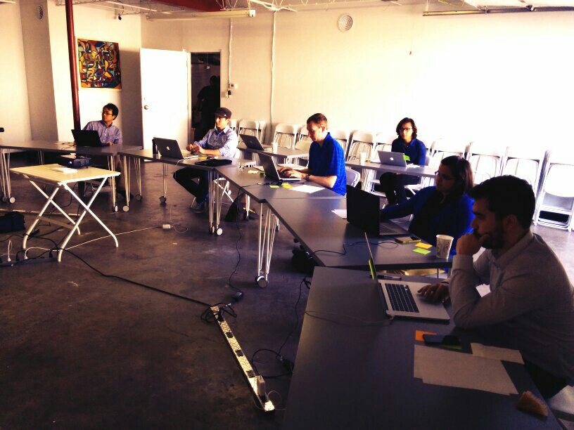
As you may know, we offer a multi-day course on 'geocomputing'. Somebody just asked me: what is this mysterious, made-up-sounding discipline? Swiftly followed by: can you really teach people how to do computational geoscience in a few days? And then: can YOU really teach people anything??

Good questions

You can come at the same kind of question from different angles. For example, sometimes professional programmers get jumpy about programming courses and the whole "learn to code" movement. I think the objection is that programming is a profession, like other kinds of engineering, and no-one would dream of offering a 3-day course on, say, dentistry for beginners.

These concerns are valid, sort of.

1. No, you can't learn to be a computational scientist in 3 days. But you can make a start. A really good one at that.
2. And no, we're not programmers. But we're scientists who get things done with code. And we're here to help.
3. And definitely no, we're not trying to teach people to be software engineers. We want to see more computational geoscientists, which is a different thing entirely.

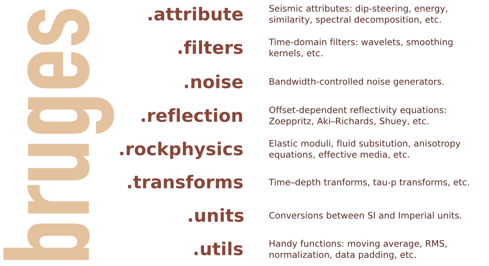
So what's geocomputing then?

Words seem inadequate for nuanced discussion. Let's instead use the language of ternary diagrams. Here's how I think 'scientific computing' stacks up against 'computer science' and 'software engineering'...

View fullsize

If you think these are confusing, just be glad I didn't go for tetrahedrons.

These are silly, of course. We could argue about them for hours I'm sure. Where would IT fit? ("It's all about the business" or something like that.) Where does Agile fit? (I've caricatured our journey, or tried to.) Where do you fit? 

SEG machine learning contest: there's still time

Have you been looking for an excuse to find out what machine learning is all about? Or maybe learn a bit of Python programming language? If so, you need to check out Brendon Hall's tutorial in the October issue of The Leading Edge. Entitled, "Facies classification using machine learning", it's a walk-through of a basic statistical learning workflow, applied to a small dataset from the Hugoton gas field in Kansas, USA.

But it was also the launch of a strictly fun contest to see who can get the best prediction from the available data. The rules are spelled out in ther contest's README, but in a nutshell, you can use any reproducible workflow you like in Python, R, Julia or Lua, and you must disclose the complete workflow. The idea is that contestants can learn from each other.

View fullsize

Left: crossplots and histograms of wireline log data, coloured by facies — the idea is to highlight possible data issues, such as highly correlated features. Right: true facies (left) and predicted facies (right) in a validation plot. See the rest of the paper for details.

What's it all about?

The task at hand is to predict sedimentological facies from well logs. Such log-derived facies are sometimes called e-facies. This is a familiar task to many development geoscientists, and there are many, many ways to go about it. In the article, Brendon trains a support vector machine to discriminate between facies. It does a fair job, but the accuracy of the result is less than 50%. The challenge of the contest is to do better.

Indeed, people have already done better; here are the current standings:

	Team	F1	Algorithm	Language	Solution
1	gccrowther	0.580	Random forest	Python	Notebook
2	LA_Team	0.568	DNN	Python	Notebook
3	gganssle	0.561	DNN	Lua	Notebook
4	MandMs	0.552	SVM	Python	Notebook
5	thanish	0.551	Random forest	R	Notebook
6	geoLEARN	0.530	Random forest	Python	Notebook
7	CannedGeo	0.512	SVM	Python	Notebook
8	BrendonHall	0.412	SVM	Python	Initial score in article

As you can see, DNNs (deep neural networks) are, in keeping with the amazing recent advances in the problem-solving capability of this technology, doing very well on this task. Of the 'shallow' methods, random forests are quite prominent, and indeed are a great first-stop for classification problems as they tend to do quite well with little tuning.

How do I enter?

There is still over 6 weeks to enter: you have until 31 January. There is a little overhead — you need to learn a bit about git and GitHub, there's some programming, and of course machine learning is a massive field to get up to speed on — but don't be discouraged. The very first entry was from Bryan Page, a self-described non-programmer who dusted off some basic skills to improve on Brendon's notebook. But you can run the notebook right here in mybinder.org (if it's up today — it's been a bit flaky lately) and a play around with a few parameters yourself.

The contest aspect is definitely low-key. There's no money on the line — just a goody bag of fun prizes and a shedload of kudos that will surely get the winners into some awesome geophysics parties. My hope is that it will encourage you (yes, you) to have fun playing with data and code, trying to do that magical thing: predict geology from geophysical data.

---

Reference

Hall, B (2016). Facies classification using machine learning. The Leading Edge 35 (10), 906–909. doi: 10.1190/tle35100906.1. (This paper is open access: you don't have to be an SEG member to read it.)

Introducing Bruges

Welcome to Bruges, a Python library (previously known as agilegeo) that contains a variety of geophysical equations used in processing, modeling and analysing seismic reflection and well log data. Here's what's in the box so far, with new stuff being added every week:

---

Simple AVO example

	VP [m/s]	VS [m/s]	ρ [kg/m3]
Rock 1	3300	1500	2400
Rock 2	3050	1400	2075

Imagine we're studying the interface between the two layers whose rock properties are shown here...

To compute the zero-offset reflection coefficient at zero offset, we pass our rock properties into the Aki-Richards equation and set the incident angle to zero:

 >>> import bruges as b
 >>> b.reflection.akirichards(vp1, vs1, rho1, vp2, vs2, rho2, theta1=0)
 -0.111995777064

Similarly, compute the reflection coefficient at 30 degrees:

 >>> b.reflection.akirichards(vp1, vs1, rho1, vp2, vs2, rho2, theta1=30)
 -0.0965206980095

To calculate the reflection coefficients for a series of angles, we can pass in a list:

 >>> b.reflection.akirichards(vp1, vs1, rho1, vp2, vs2, rho2, theta1=[0,10,20,30])
 [-0.11199578 -0.10982911 -0.10398651 -0.0965207 ]

Similarly, we could compute all the reflection coefficients for all incidence angles from 0 to 70 degrees, in one degree increments, by passing in a range:

 >>> b.reflection.akirichards(vp1, vs1, rho1, vp2, vs2, rho2, theta1=range(70))
 [-0.11199578 -0.11197358 -0.11190703 ... -0.16646998 -0.17619878 -0.18696428]

A few more lines of code, shown in the Jupyter notebook, and we can make some plots:

---

Elastic moduli calculations

With the same set of rocks in the table above we could quickly calculate the Lamé parameters λ and µ, say for the first rock, like so (in SI units),

 >>> b.rockphysics.lam(vp1, vs1, rho1), b.rockphysics.mu(vp1, vs1, rho1)
 15336000000.0 5400000000.0

Sure, the equations for λ and µ in terms of P-wave velocity, S-wave velocity, and density are pretty straightforward: 

but there are many other elastic moduli formulations that aren't. Bruges knows all of them, even the weird ones in terms of E and λ.

---

All of these examples, and lots of others — Backus averaging,  examples are available in this Jupyter notebook, if you'd like to work through them on your own.

---

Bruges is a...

It is very much early days for Bruges, but the goal is to expose all the geophysical equations that geophysicists like us depend on in their daily work. If you can't find what you're looking for, tell us what's missing, and together, we'll make it grow.

What's a handy geophysical equation that you employ in your work? Let us know in the comments!

Geocomputing: Call for papers

52 Things .+? Geocomputing is in the works.

For previous books, we've reached out to people we know and trust. This felt like the right way to start our micropublishing project, because we had zero credibility as publishers, and were asking a lot from people to believe anything would come of it.

Now we know we can do it, but personal invitation means writing to a lot of people. We only hear back from about 50% of everyone we write to, and only about 50% of those ever submit anything. So each book takes about 160 invitations.

This time, I'd like to try something different, and see if we can truly crowdsource these books. If you would like to write a short contribution for this book on geoscience and computing, please have a look at the author guidelines. In a nutshell, we need about 600 words before the end of March. A figure or two is OK, and code is very much encouraged. Publication date: fall 2015.

We would also like to find some reviewers. If you would be available to read at least 5 essays, and provide feedback to us and the authors, please let me know. 

In keeping with past practice, we will be donating money from sales of the book to scientific Python community projects via the non-profit NumFOCUS Foundation.

What the cover might look like. If you'd like to write for us, please read the author guidelines.

How much rock was erupted from Mt St Helens?

One of the reasons we struggle when learning a new skill is not necessarily because this thing is inherently hard, or that we are dim. We just don't yet have enough context for all the connecting ideas to, well, connect. With this in mind I wrote this introductory demo for my Creative Geocomputing class, and tried it out in the garage attached to START Houston, when we ran the course there a few weeks ago.

I walked through the process of transforming USGS text files to data graphics. The motivation was to try to answer the question: How much rock was erupted from Mount St Helens?

This gorgeous data set can be reworked to serve a lot of programming and data manipulation practice, and just have fun solving problems. My goal was to maintain a coherent stream of instructions, especially for folks who have never written a line of code before. The challenge, I found, is anticipating when words, phrases, and syntax are being heard like a foriegn language (as indeed they are), and to cope by augmenting with spoken narrative.

Text file to 3D plot

To start, we'll import a code library called NumPy that's great for crunching numbers, and we'll abbreviate it with the nickname np:

>>> import numpy as np

Then we can use one of its functions to load the text file into an array we'll call data:

>>> data = np.loadtxt('z_after.txt')

The variable data is a 2-dimensional array (matrix) of numbers. It has an attribute that we can call upon, called shape, that holds the number of elements it has in each dimension,

>>> data.shape
(1370, 949)

If we want to make a plot of this data, we might want to take a look at the range of the elements in the array, we can call the peak-to-peak method on data,

>>> data.ptp()
41134.0

Whoa, something's not right, there's not a surface on earth that has a min to max elevation that large. Let's dig a little deeper. The highest point on the surface is,

>>> np.amax(data)
8367.0

Which looks to the adequately trained eye like a reasonable elevation value with units of feet. Let's look at the minimum value of the array,

>>> np.amin(data)
-32767.0 

OK, here's the problem. GIS people might recognize this as a null value for elevation data, but since we aren't assuming any knowledge of GIS formats and data standards, we can simply replace the values in the array with not-a-number (NaN), so they won't contaminate our plot.

>>> data[data==-32767.0] = np.nan

To view this surface in 3D we can import the mlab module from Mayavi, 

>>> from mayavi import mlab

Finally we call the surface function from mlab, and pass the input data, and a colormap keyword to activate a geographically inspired colormap, and a vertical scale coefficient.

>>> mlab.surf(data,
              colormap='gist_earth',
              warp_scale=0.05)

After applying the same procedure to the pre-eruption digits, we're ready to do some calculations and visualize the result to reveal the output and its fascinating characteristics. Read more in the IPython Notebook.

If this 10 minute introduction is compelling and you'd like to learn how to wrangle data like this, sign up for the two-day version of this course next week in Calgary.