What is scientific computing?

I started my career in sequence stratigraphy, so I know a futile discussion about semantics when I see one. But humour me for a second.

As you may know, we offer a multi-day course on 'geocomputing'. Somebody just asked me: what is this mysterious, made-up-sounding discipline? Swiftly followed by: can you really teach people how to do computational geoscience in a few days? And then: can YOU really teach people anything??

Good questions

You can come at the same kind of question from different angles. For example, sometimes professional programmers get jumpy about programming courses and the whole "learn to code" movement. I think the objection is that programming is a profession, like other kinds of engineering, and no-one would dream of offering a 3-day course on, say, dentistry for beginners.

These concerns are valid, sort of.

  1. No, you can't learn to be a computational scientist in 3 days. But you can make a start. A really good one at that.
  2. And no, we're not programmers. But we're scientists who get things done with code. And we're here to help.
  3. And definitely no, we're not trying to teach people to be software engineers. We want to see more computational geoscientists, which is a different thing entirely.

So what's geocomputing then?

Words seem inadequate for nuanced discussion. Let's instead use the language of ternary diagrams. Here's how I think 'scientific computing' stacks up against 'computer science' and 'software engineering'...

If you think these are confusing, just be glad I didn't go for tetrahedrons.

These are silly, of course. We could argue about them for hours I'm sure. Where would IT fit? ("It's all about the business" or something like that.) Where does Agile fit? (I've caricatured our journey, or tried to.) Where do you fit? 

Not getting hacked

This kind of password is horrible for lots of reasons. The real solution to password madness is a password manager.

This kind of password is horrible for lots of reasons. The real solution to password madness is a password manager.

The end of the year is a great time to look around at your life and sort stuff out. One of the things you almost certainly need to sort out is your online security. Because if you haven't been hacked already (you probably have), you're just about to be.

Just look at some recent stories from the world of data security:

There are plenty of others; Wired has been keeping track of them — read more here. Or check out Wikipedia's list.

Despite all this, I see hardly anyone using a password manager, and anecdotally I hear that hardly anyone uses two-factor authentication either. This tells me that at least 80% of smart people, inlcuding lots of my friends and relatives, are in daily peril. Oh no!

After reading this post, I hope you do two things:

  • Start using a password manager. If you only do one thing, do this.
  • Turn on two-factor authentication for your most vulnerable accounts.

Start using a password manager

Please, right now, download and install LastPass on every device and in every browser you use. It's awesome:

  • It stores all your passwords! This way, they can all be different, and each one can be highly secure.
  • It generates secure, random passwords for new accounts you create. 
  • It scores you on the security level of your passwords, and lets you easily change insecure ones.
  • The free version is awesome, and the premium version is only $2/month.

There are other password managers, of course, but I've used this one for years and it's excellent. Once you're set up, you can start changing passwords that are insecure, or re-used on multiple sites... or which are at Uber, Yahoo, or Equifax.

One surprise from using LastPass is being able to count the number of accounts I have created around the web over the years. I have 473 accounts stored in LastPass! That's 473 places to get hacked... how many places are you exposed?

The one catch: you need a bulletproof key for your password manager. Best advice: use a long pass-phrase instead.

The obligatory password cartoon, by xkcd and licensed CC-BY-NC

The obligatory password cartoon, by xkcd and licensed CC-BY-NC

authenticator.png

Two-factor authentication

Sure, it's belt and braces — but you don't want your security trousers to fall down, right? 

Er, anyway, the point is that even with a secure password, your password can still be stolen and your account compromised. But it's much, much harder if you use two-factor authentication, aka 2FA. This requires you to enter a code — from a hardware key or an app, or received via SMS — as well as your password. If you use an app, it introduces still another layer of security, because your phone should be locked.

I use Google's Authenticator app, and I like it. There's a little bit of hassle the first time you set it up, but after that it's plain sailing. I have 2FA turned on for all my 'high risk' accounts: Google, Twitter, Facebook, Apple, AWS, my credit card processor, my accounting software, my bank, my domain name provider, GitHub, and of course LastPass. Indeed, LastPass even lets me specify that logins must originate in Canada. 

What else can you do?

There are some other easy things you can do to make yourself less hackable:

  • Install updates on your phones, tablets, and other computers. Keep browsers and operating systems up to date.
  • Be on high alert for phishing attempts. Don't follow links to sites like your bank or social media sites — type them into your browser if possible. Be very suspicious of anyone contacting you, especially banks.
  • Don't use USB sticks. The cloud is much safer — I use Dropbox myself, it's awesome.

For more tips, check out this excellent article from Motherboard on not getting hacked.

The norm and simple solutions

Last time I wrote about different ways of calculating distance in a vector space — say, a two-dimensional Euclidean plane like the streets of Portland, Oregon. I showed three ways to reckon the distance, or norm, between two points (i.e. vectors). As a reminder, using the distance between points u and v on the map below this time:

$$ \|\mathbf{u} - \mathbf{v}\|_1 = |u_x - v_x| + |u_y - v_y| $$

$$ \|\mathbf{u} - \mathbf{v}\|_2 = \sqrt{(u_x - v_x)^2 + (u_y - v_y)^2} $$

$$ \|\mathbf{u} - \mathbf{v}\|_\infty = \mathrm{max}(|u_x - v_x|, |u_y - v_y|) $$

Let's think about all the other points on Portland's streets that are the same distance away from u as v is. Again, we have to think about what we mean by distance. If we're walking, or taking a cab, we'll need to think about \(\ell_1\) — the sum of the distances in x and y. This is shown on the left-most map, below.

For simplicity, imagine u is the origin, or (0, 0) in Cartesian coordinates. Then v is (0, 4). The sum of the distances is 4. Looking for points with the same sum, we find the pink points on the map.

If we're thinking about how the crow flies, or \(\ell_2\) norm, then the middle map sums up the situation: the pink points are all equidistant from u. All good: this is what we usually think of as 'distance'.

norms_equidistant_L0.png

The \(\ell_\infty\) norm, on the other hand, only cares about the maximum distance in any direction, or the maximum element in the vector. So all points whose maximum coordinate is 4 meet the criterion: (1, 4), (2, 4), (4, 3) and (4, 0) all work.

You might remember there was also a weird definition for the \(\ell_0\) norm, which basically just counts the non-zero elements of the vector. So, again treating u as the origin for simplicity, we're looking for all the points that, like v, have only one non-zero Cartesian coordinate. These points form an upright cross, like a + sign (right).

So there you have it: four ways to draw a circle.

Wait, what?

A circle is just a set of points that are equidistant from the centre. So, depending on how you define distance, the shapes above are all 'circles'. In particular, if we normalize the (u, v) distance as 1, we have the following unit circles:

It turns out we can define any number of norms (if you like the sound of \(\ell_{2.4}\) or \(\ell_{240}\) or \(\ell_{0.024}\)...) but most of the time, these will suffice. You can probably imagine the shapes of the unit circles defined by these other norms.

What can we do with this stuff?

Let's think about solving equations. Think about solving this:

$$ x + 2y = 8 $$

norms_line.png

I'm sure you can come up with a soluiton in your head, x = 6 and y = 1 maybe. But one equation and two unknowns means that this problem is underdetermined, and consequently has an infinite number of solutions. The solutions can be visualized geometrically as a line in the Euclidean plane (right).

But let's say I don't want solutions like (3.141590, 2.429205) or (2742, –1367). Let's say I want the simplest solution. What's the simplest solution?

norms_line_l2.png

This is a reasonable question, but how we answer it depends how we define 'simple'. One way is to ask for the nearest solution to the origin. Also reasonable... but remember that we have a few different ways to define 'nearest'. Let's start with the everyday definition: the shortest crow-flies distance from the origin. The crow-flies, \(\ell_2\) distances all lie on a circle, so you can imagine starting with a tiny circle at the origin, and 'inflating' it until it touches the line \(x + 2y - 8 = 0\). This is usually called the minimum norm solution, minimized on \(\ell_2\). We can find it in Python like so:

    import numpy.linalg as la
    A = [[1, 2]]
    b = [8]
    la.lstsq(A, b)

The result is the vector (1.6, 3.2). You could almost have worked that out in your head, but imagine having 1000 equations to solve and you start to appreciate numpy.linalg. Admittedly, it's even easier in Octave (or MATLAB if you must) and Julia:

    A = [1 2]
    b = [8]
    A \ b
norms_line_all.png

But remember we have lots of norms. It turns out that minimizing other norms can be really useful. For example, minimizing the \(\ell_1\) norm — growing a diamond out from the origin — results in (0, 4). The \(\ell_0\) norm gives the same sparse* result. Minimizing the \(\ell_\infty\) norm leads to \( x = y = 8/3 \approx 2.67\).

This was the diagram I wanted to get to when I started with the 'how far away is the supermarket' business. So I think I'll stop now... have fun with Norm!


* I won't get into sparsity now, but it's a big deal. People doing big computations are always looking for sparse representations of things. They use less memory, are less expensive to compute with, and are conceptually 'neater'. Sparsity is really important in compressed sensing, which has been a bit of a buzzword in geophysics lately.

The norm: kings, crows and taxicabs

How far away is the supermarket from your house? There are lots of ways of answering this question:

  • As the crow flies. This is the green line from \(\mathbf{a}\) to \(\mathbf{b}\) on the map below.

  • The 'city block' driving distance. If you live on a grid of streets, all possible routes are the same length — represented by the orange lines on the map below.

  • In time, not distance. This is usually a more useful answer... but not one we're going to discuss today.

Don't worry about the mathematical notation on this map just yet. The point is that there's more than one way to think about the distance between two points, or indeed any measure of 'size'.

norms.png

Higher dimensions

The map is obviously two-dimensional, but it's fairly easy to conceive of 'size' in any number of dimensions. This is important, because we often deal with more than the 2 dimensions on a map, or even the 3 dimensions of a seismic stack. For example, we think of raw so-called 3D seismic data as having 5 dimensions (x position, y position, offset, time, and azimuth). We might even formulate a machine learning task with a hundred or more dimensions (or 'features').

Why do we care about measuring distances in high dimensions? When we're dealing with data in these high-dimensional spaces, 'distance' is a useful way to measure the similarity between two points. For example, I might want to select those samples that are close to a particular point of interest. Or, from among the points satisfying some constraint, select the one that's closest to the origin.

Definitions and nomenclature

We'll define norms in the context of linear algebra, which is the study of vector spaces (think of multi-dimensional 'data spaces' like the 5D space of seismic data). A norm is a function that assigns a positive scalar size to a vector \(\mathbf{v}\) , with a size of zero reserved for the zero vector (in the Cartesian plane, the zero vector has coordinates (0, 0) and is usually called the origin). Any norm \(\|\mathbf{v}\|\) of this vector satisfies the following conditions:

  1. Absolutely homogenous. The norm of \(\alpha\mathbf{v}\) is equal to \(|\alpha|\) times the norm of \(\mathbf{v}\).

  2. Subadditive. The norm of \( (\mathbf{u} + \mathbf{v}) \) is less than or equal to the norm of \(\mathbf{u}\) plus the norm of \(\mathbf{v}\). In other words, the norm satisfies the triangle inequality.

  3. Positive. The first two conditions imply that the norm is non-negative.

  4. Definite. Only the zero vector has a norm of 0.

Kings, crows and taxicabs

Let's return to the point about lots of ways to define distance. We'll start with the most familiar definition of distance on a map— the Euclidean distance, aka the \(\ell_2\) or \(L_2\) norm (confusingly, sometimes the two is written as a superscript), the 2-norm, or sometimes just 'the norm' (who says maths has too much jargon?). This is the 'as-the-crow-flies distance' on the map above, and we can calculate it using Pythagoras:

$$ \|\mathbf{v}\|_2 = \sqrt{(a_x - b_x)^2 + (a_y - b_y)^2} $$

You can extend this to an arbitrary number of dimensions, just keep adding the squared elementwise differences. We can also calculate the norm of a single vector in n-space, which is really just the distance between the origin and the vector:

$$ \|\mathbf{u}\|_2 = \sqrt{u_1^2 + u_2^2 + \ldots + u_n^2}  = \sqrt{\mathbf{u} \cdot \mathbf{u}} $$

As shown here, the 2-norm of a vector is the square root of its dot product with itself.

So the crow-flies distance is fairly intuitive... what about that awkward city block distance? This is usually referred to as the Manhattan distance, the taxicab distance, the \(\ell_1\) or \(L_1\) norm, or the 1-norm. As you can see on the map, it's just the sum of the absolute distances in each dimension, x and y in our case:

$$ \|\mathbf{v}\|_1 = |a_x - b_x| + |a_y - b_y| $$

What's this magic number 1 all about? It turns out that the distance metric can be generalized as the so-called p-norm, where p can take any positive value up to infinity. The definition of the p-norm is consistent with the two norms we just met:

$$ \| \mathbf{u} \|_p = \left( \sum_{i=1}^n | u_i | ^p \right)^{1/p} $$

[EDIT, May 2021: This generalized version is sometimes called the Minkowski distance, e.g. in the scipy documentation.]

In practice, I've only ever seen p = 1, 2, or infinity (and 0, but we'll get to that). Let's look at the meaning of the \(\infty\)-norm, aka the \(\ell_\infty\) or \(L_\infty\) norm, which is sometimes called the Chebyshev distance or chessboard distance (because it defines the minimum number of moves for a king to any given square):

$$ \|\mathbf{v}\|_\infty = \mathrm{max}(|a_x - b_x|, |a_y - b_y|) $$

In other words, the Chebyshev distance is simply the maximum element in a given vector. In a nutshell, the infinitieth root of the sum of a bunch of numbers raised to the infinitieth power, is the same as the infinitieth root of the largest of those numbers raised to the infinitieth power — because infinity is weird like that.

What about p = 0?

Infinity is weird, but so is zero sometimes. Taking the zeroeth root of a lot of ones doesn't make a lot of sense, so mathematicians often redefine the \(\ell_0\) or \(L_0\) "norm" (not a true norm) as a simple count of the number of non-zero elements in a vector. In other words, we toss out the 0th root, define \(0^0 := 0 \) and do:

$$ \| \mathbf{u} \|_0 = |u_1|^0 + |u_2|^0 + \cdots + |u_n|^0 $$

(Or, if we're thinking about the points \(\mathbf{a}\) and \(\mathbf{b}\) again, just remember that \(\mathbf{v}\) = \(\mathbf{a}\) - \(\mathbf{b}\).)

Computing norms

Let's take a quick look at computing the norm of some vectors in Python:

 
>>> import numpy as np

>>> a = np.array([1, 1]).T
>>> b = np.array([6, 5]).T

>>> L_0 = np.count_nonzero(a - b)
2

>>> L_1 = np.sum(np.abs(a - b))
9

>>> L_2 = np.sqrt((a - b) @ (a - b))
6.4031242374328485

>>> L_inf = np.max(np.abs(a - b))
5

>>> # Using NumPy's `linalg` module:
>>> import numpy.linalg as la
>>> for p in (0, 1, 2, np.inf):
>>>    print("L_{} norm = {}".format(p, la.norm(a - b, p)))
L_0 norm = 2.0
L_1 norm = 9.0
L_2 norm = 6.4031242374328485
L_inf norm = 5.0

What can we do with all this?

So far, so good. But what's the point of these metrics? How can we use them to solve problems? We'll get into that in a future post, so don't go too far!

For now I'll leave you to play with this little interactive demo of the effect of changing p-norms on a Voronoi triangle tiling — it's by Sarah Greer, a geophysics student at UT Austin. 


UPDATE — The next post is The norm and simple solutions, which looks at how these different norms can be used to solve real-world problems.

Machine learning and analytics in geoscience

We're at EAGE in Paris. I'm sitting in a corner of the exhibition because the power is out in the main hall, so all the talks for the afternoon have been postponed. The poor EAGE team must be beside themselves, I feel for them. (Note to future event organizers: white boards!)

Yesterday Diego, Evan, and I — along with lots of hackathon participants — were at the Data Science for Geosciences workshop, an all-day machine learning fest. The session was chaired by Cyril Agut (Total), Marianne Cuif-Sjostrand (Total), Florence Delprat-Jannaud (IFPEN), and Noalwenn Dubos-Sallée (IFPEN), and they had assembled a good programme, with quite a bit of variety.

Michel Lutz, Group Data Officer at Total, and adjunct at École des Mines de Saint-Étienne, gave a talk entitled, Data science & application to geosciences: an introduction. It was high-level but thoughtful, and such glimpses into large companies are always interesting. The company seems to have a mature data science strategy, and a well-developed technology stack. Henri Blondelle (AgileDD) asked about open data at the end, and Michel somewhat sidestepped on specifics, but at least conceded that the company could do more in open source code, if not data.

Infrastructure, big data, and IoT

Next we heard a set of talks about the infrastructure aspect of big (really big) data.

Alan Smith of Luchelan told the group about some negative experiences with Hadoop and seismic data (though it didn't seem to me that his problems were insoluble since I know of several projects that use it), and the realization that sometimes you just need fast infrastructure and custom software.

Hadi Jamali-Rad of Shell followed with an IoT story from the field. He had deployed a large number of wireless seismic sensors around a village in Holland, then tested various aspects of the communication system to answer questions like, what's the packet loss rate when you collect data from the nodes? What about from a balloon stationed over the site?

Duncan Irving of Teradata asked, Why aren't we [in geoscience] doing live analytics on 100PB of live data like eBay? His hypothesis is that IT organizations in oil and gas failed to keep up with key developments in data analytics, so now there's a crisis of sorts and we need to change how we handle our processes and culture around big data. 

Machine learning

We shifted gears a bit after lunch. I started with a characteristically meta talk about how I think our community can help ensure that our research and practice in this domain leads to good places as soon as possible. I'll record it and post it soon.

Nicolas Audebert of ONERA/IRISA presented a nice application of a 3D convolutional neural network (CNN) to the segmentation and classification of hyperspectral aerial photography. His images have between about 100 and 400 channels, and he finds that CNNs reduce error rates by up to about 50% (compared to an SVM) on noisy or complex images. 

Henri Blondelle of Agile Data Decisions talked about his experience of the CDA's unstructured data challenge of 2016. About 80% of the dataset is unstructured (e.g. folders of PDFs and TIFFs), and Henri's vision is to transform 80% of that into structured data, using tools like AgileDD's IQC to do OCR and heuristic labeling. 

Irina Emelyanova of CSIRO provided another case study: unsupervised e-facies prediction using various types of clustering, from K-means to some interesting variants of self-organizing maps. It was refreshing to see someone revealing a lot of the details of their implementation.

Jan Limbeck, a research scientist at Shell wrapped up the session with an overview of Shell's activities around big data and machine learning, as they prepare for exabytes. He mentioned the Mauricio Araya-Polo et al. paper on deep learning in seismic shot gathers in the special March issue of The Leading Edge — clearly it's easiest to talk about things they've already published. He also listed a lot of Shell's machine learning projects (frac optimization, knowledge graphs, reservoir simulation, etc), but there's no way to know what state they are in or what their chances of success are. 

As well as all the 9 talks, there were 13 posters, about a third of which were on infrastructure stuff, with the rest providing more case studies. Unfortunately, I didn't get the chance to look at them in any detail, but I appreciated the organizers making time for discussion around the posters. If they'd also allowed more physical space for the discussion it could have been awesome.

Analytics!

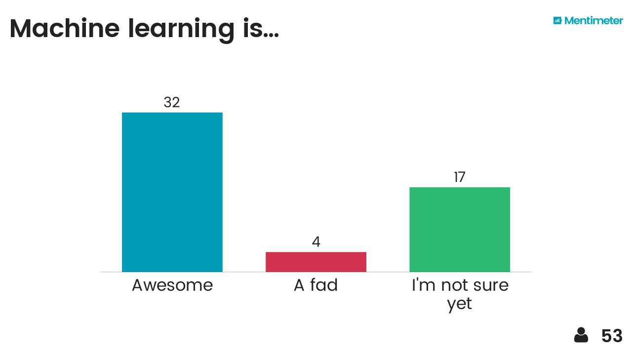
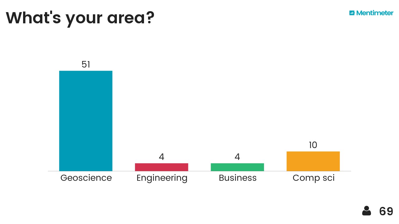
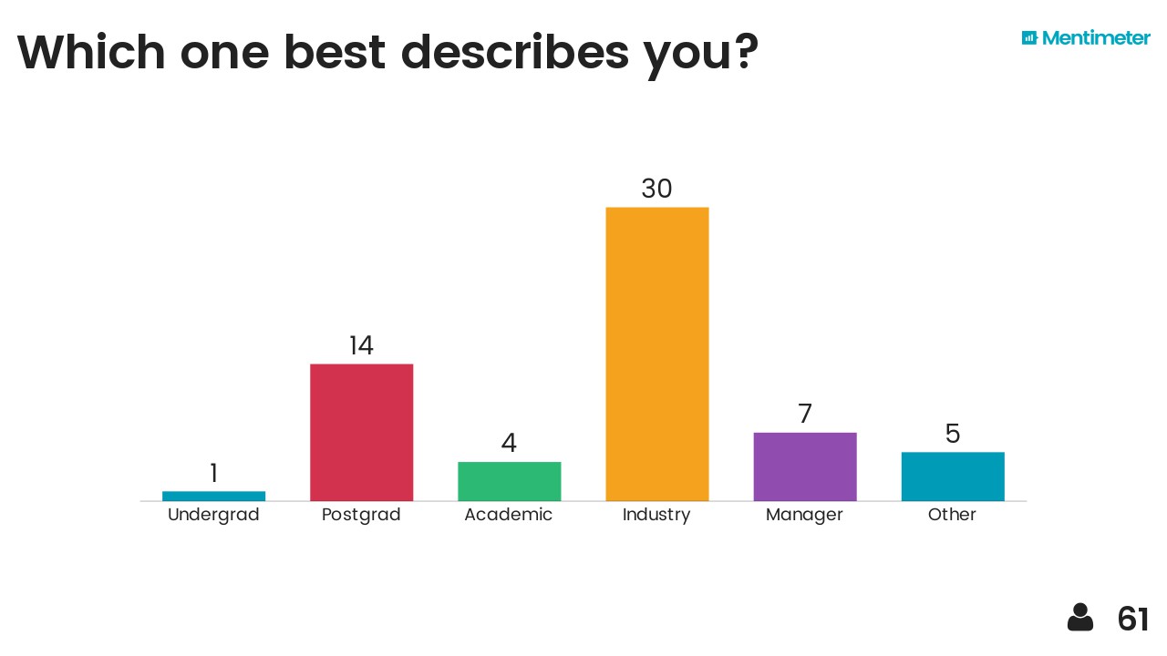
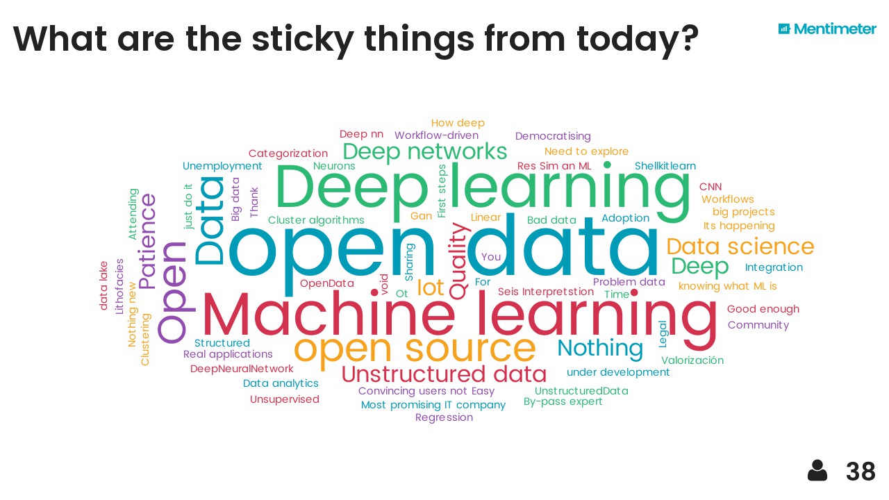
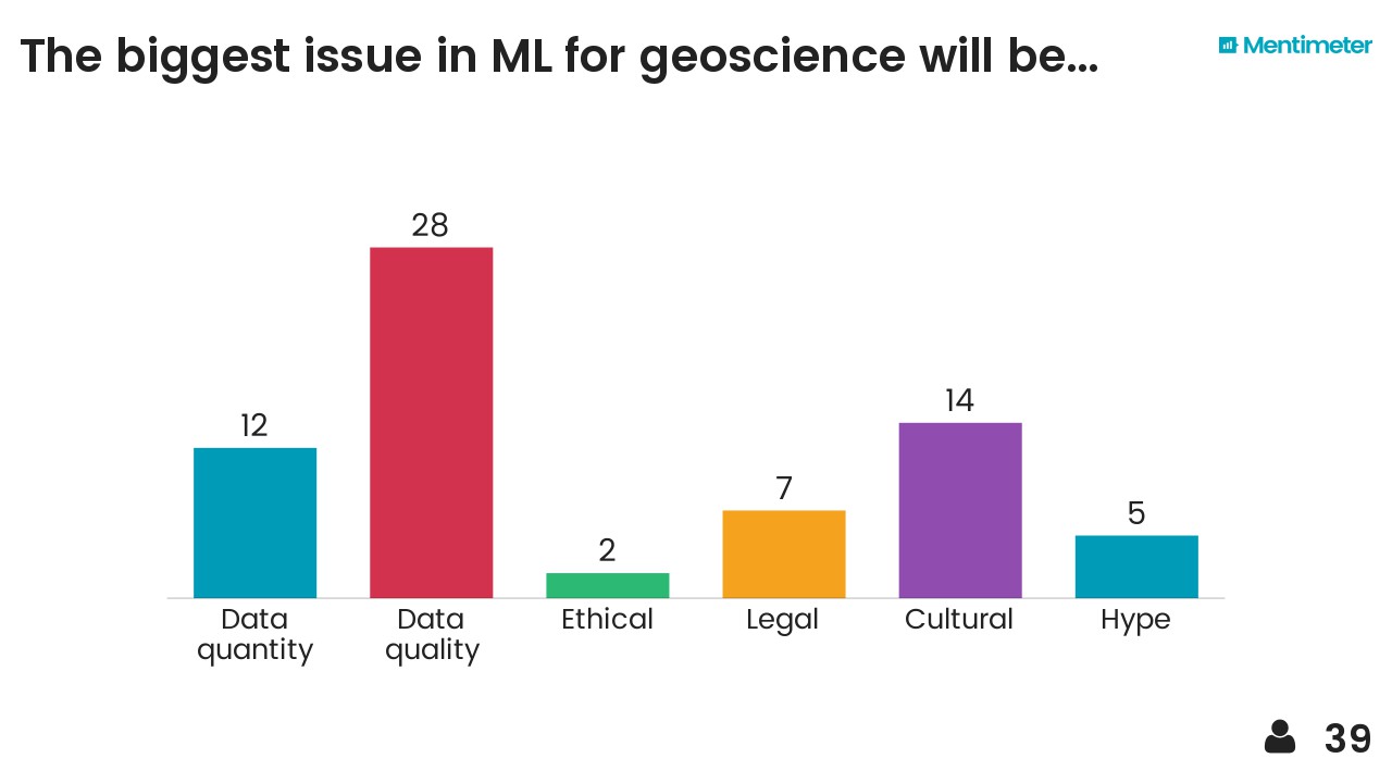
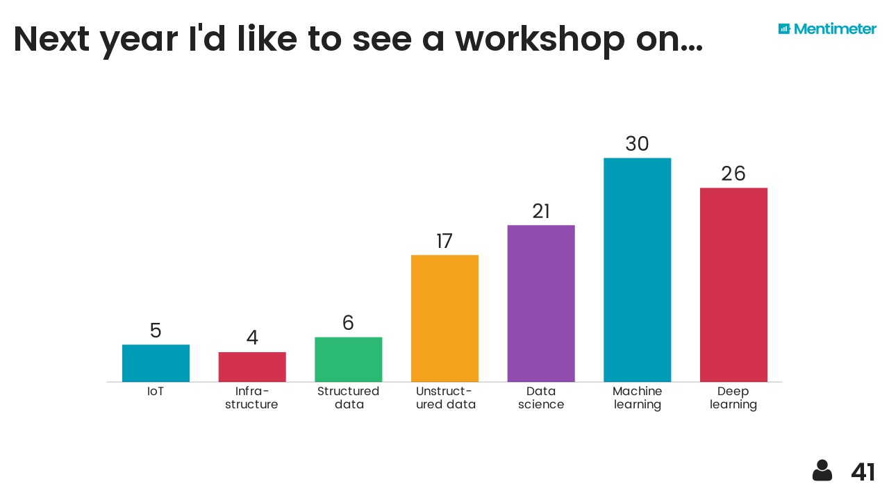
After hearing about Mentimeter from Chris Jackson I took the opportunity to try it out on the audience. Here are the results, I think they are fairly self-explanatory... 

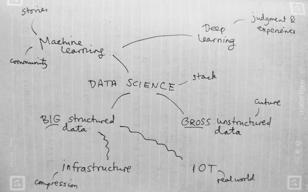
I also threw in the mindmap I drew at the end as a sort of summary. The vertical axis represents something like'abstraction' or 'time' (in a workflow sense) and I think each layer depends somewhat on those beneath it. It probably makes sense to no-one but me.

Breakout!

It seems clear that 2017 is the breakout year for machine learning in petroleum geoscience, and in petroleum in general. If your company or institution has not yet gone beyond "watching" or "thinking about" data science and machine learning, then it is falling behind by a little more every day, and it has been for at least a year. Now's the time to choose if you want to be part of what happens next, or a victim of it.

The Computer History Museum

Mountain View, California, looking northeast over US 101 and San Francisco Bay. The Computer History Museum sits between the Googleplex and NASA Ames. Hangar 1, the giant airship hangar, is visible on the right of the image. Imagery and map data © Google, Landsat/Copernicus.

A few days ago I was lucky enough to have a client meeting in Santa Clara, California. I had not been to Silicon Valley before, and it was more than a little exciting to drive down US Route 101 past the offices of Google, Oracle and Amazon and basically every other tech company, marvelling at Intel’s factory and the hangars at NASA Ames, and seeing signs to places like Stanford, Mountain View, and Menlo Park.

I had a spare day before I flew home, and decided to visit Stanford’s legendary geophysics department, where there was a lecture that day. With an hour or so to kill, I thought I’d take in the Computer History Museum on the way… I never made it to Stanford.

The museum

The Computer History Museum was founded in 1996, building on an ambition of über-geek Gordon Bell. It sits in the heart of Mountain View, surrounded by the Googleplex, NASA Ames, and Microsoft. It’s a modern, airy building with the museum and a small café downstairs, and meeting facilities on the upper floor. It turns out to be an easy place to burn four hours.

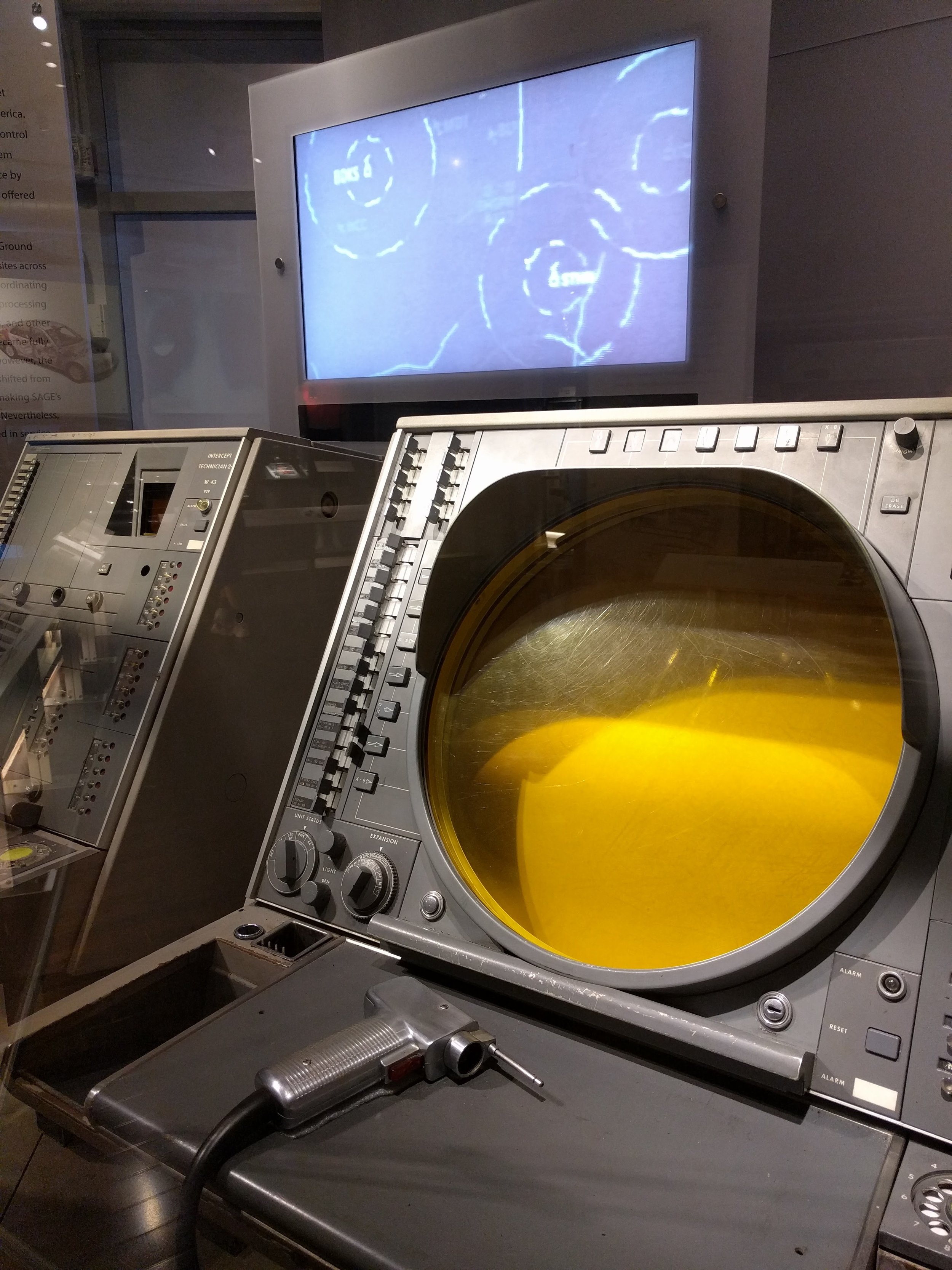
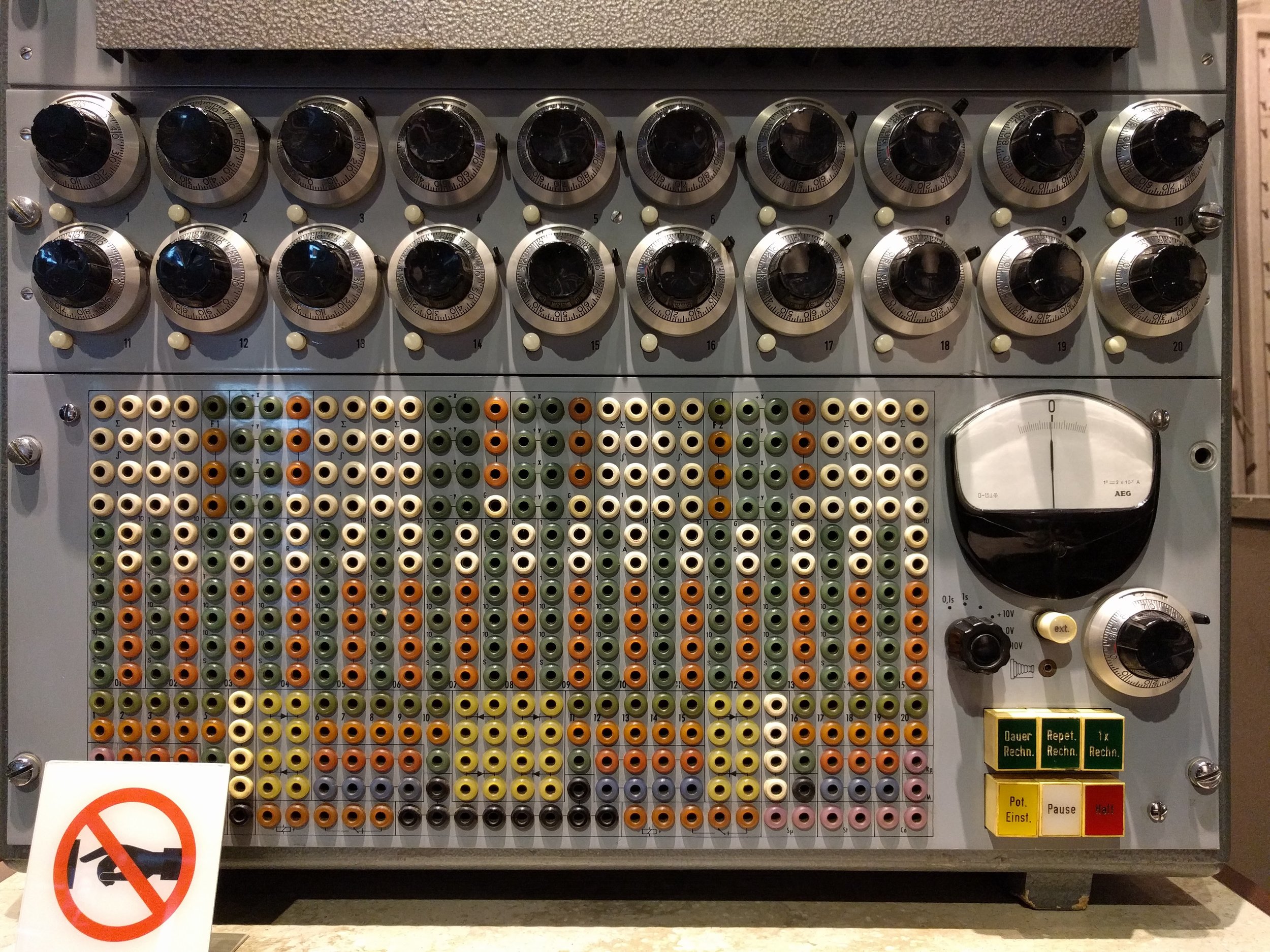
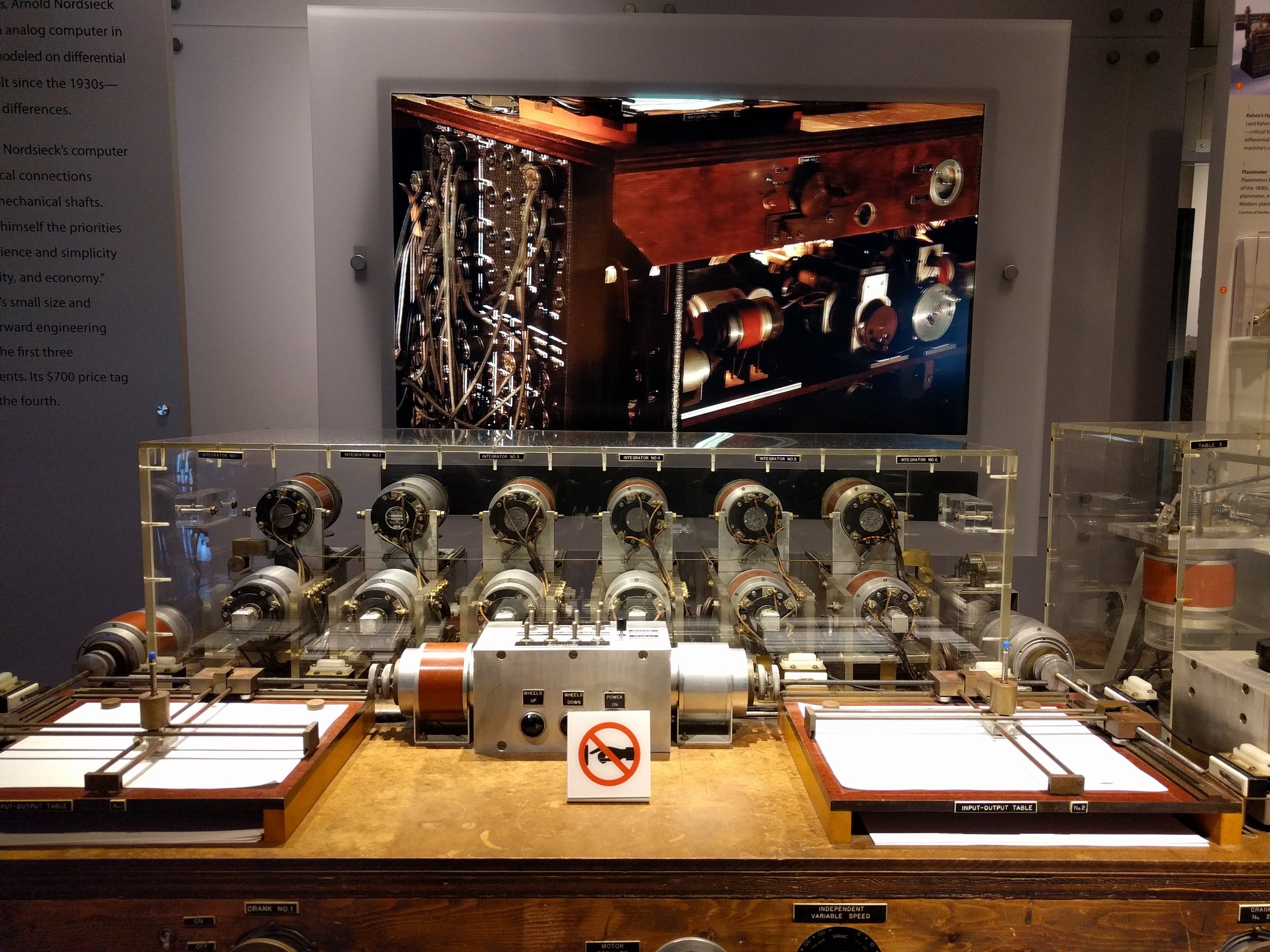
I saw a lot of computers that day. You can see them too because much of the collection is in the online catalog. A few things that stood out for me were:

No seismic

I had been hoping to read more about the early days of Texas Instruments, because it was spun out of a seismic company, Geophysical Service or GSI, and at least some of their early integrated circuit research was driven by the needs of seismic imaging. But I was surprised not to find a single mention of seismic processing in the place. We should help them fix this!

SEG-Y Rev 2 again: little-endian is legal!
Big news! Little-endian byte order is finally legal in SEG-Y files.

That's not all. I already spilled the beans on 64-bit floats. You can now have up to 18 quintillion traces (18 exatraces?) in a seismic line. And, finally, the hyphen confusion is cleared up: it's 'SEG-Y', with a hyphen. All this is spelled out in the new SEG-Y specification, Revision 2.0, which was officially released yesterday after at least five years in the making. Congratulations to Jill Lewis, Rune Hagelund, Stewart Levin, and the rest of the SEG Technical Standards Committee

Back up a sec: what's an endian?

Whenever you have to think about the order of bytes (the 8-bit chunks in a 'word' of 32 bits, for example) — for instance when you send data down a wire, or store bytes in memory, or in a file on disk — you have to decide if you're Roman Catholic or Church of England.

What?

It's not really about religion. It's about eggs.

In one of the more obscure satirical analogies in English literature, Jonathan Swift wrote about the ideological tussle between between two factions of Lilliputians in Gulliver's Travels (1726). The Big-Endians liked to break their eggs at the big end, while the Little-Endians preferred the pointier option. Chaos ensued.

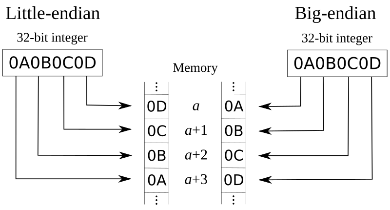
Two hundred and fifty years later, Danny Cohen borrowed the terminology in his 1 April 1980 paper, On Holy Wars and a Plea for Peace — in which he positioned the Big-Endians, preferring to store the big bytes first in memory, against the Little-Endians, who naturally prefer to store the little ones first. Big bytes first is how the Internet shuttles data around, so big-endian is sometimes called network byte order. The drawing (right) shows how the 4 bytes in a 32-bit 'word' (the hexadecimal codes 0A, 0B, 0C and 0D) sit in memory.

Because we write ordinary numbers big-endian style — 2017 has the thousands first, the units last — big-endian might seem intuitive. Then again, lots of people write dates as, say, 31-03-2017, which is analogous to little-endian order. Cohen reviews the computational considerations in his paper, but really these are just conventions. Some architectures pick one, some pick the other. It just happens that the x86 architecture that powers most desktop and laptop computers is little-endian, so people have been illegally (and often accidentally) writing little-endian SEG-Y files for ages. Now it's actually allowed.

Still other byte orders are possible. Some processors, notably ARM and other RISC architectures, are middle-endian (aka mixed endian or bi-endian). You can think of this as analogous to the month-first American date format: 03-31-2017. For example, the two halves of a 32-bit word might be reversed compared to their 'pure' endian order. I guess this is like breaking your boiled egg in the middle. Swift did not tell us which religious denomination these hapless folks subscribe to.

OK, that's enough about byte order

I agree. So I'll end with this handy SEG-Y cheatsheet. Click here for the PDF.


References and acknowledgments

Cohen, Danny (April 1, 1980). On Holy Wars and a Plea for PeaceIETF. IEN 137. "...which bit should travel first, the bit from the little end of the word, or the bit from the big end of the word? The followers of the former approach are called the Little-Endians, and the followers of the latter are called the Big-Endians." Also published at IEEE ComputerOctober 1981 issue.

Thumbnail image: “Remember, people will judge you by your actions, not your intentions. You may have a heart of gold -- but so does a hard-boiled egg.” by Kate Ter Haar is licensed under CC BY 2.0

More precise SEG-Y?

The impending SEG-Y Revision 2 release allows the use of double-precision floating point numbers. This news might leave some people thinking: "What?".

Integers and floats

In most computing environments, there are various kinds of number. The main two are integers and floating point numbers. Let's take a quick look at integers, or ints, first.

Integers can only represent round numbers: 0, 1, 2, 3, etc. They can have two main flavours: signed and unsigned, and various bit-depths, e.g. 8-bit, 16-bit, and so on. An 8-bit unsigned integer can have values between 0 and 255; signed ints go from -128 to +127 using a mathematical operation called two's complement.

As you might guess, floating point numbers, or floats, are used to represent all the other numbers — you know, numbers like 4.1 and –7.2346312 × 10¹³ — we need lots of those.  

Floats in binary

OK, so we need to know about floats. To understand what double-precision means, we need to know how floats are represented in computers. In other words, how on earth can a binary number like 01000010011011001010110100010101 represent a floating point number?

It's fairly easy to understand how integers are stored in binary: the 8-bit binary number 01001101 is the integer 77 in decimal, or 4D in hexadecimal; 11111111 is 255 (base 10) or FF (base 16) if we're dealing with unsigned ints, or -1 decimal if we're in the two's complement realm of signed ints.

Clearly we can only represent a certain number of values with, say, 16 bits. This would give us 65 536 integers... but that's not enough dynamic range represent tiny or gigantic floats, not if we want any precision at all. So we have a bit of a paradox: we'd like to represent a huge range of numbers (down around the mass of an electron, say, and up to Avogadro's number), but with reasonably high precision, at least a few significant figures. This is where floating point representations come in.

Scientific notation, sort of

If you're thinking about scientific notation, you're thinking on the right lines. We raise some base (say, 10) to some integer exponent, and multiply by another integer (called the mantissa, or significand). That way, we can write a huge range of numbers with plenty of precision, using only two integers. So:

$$ 3.14159 = 314159 \times 10^{-5} \ \ \mathrm{and} \ \ 6.02214 \times 10^{23} = 602214 \times 10^{18} $$

If I have two bytes at my disposal (so-called 'half precision'), I could have an 8-bit int for the integer part, called the significand, and another 8-bit int for the exponent. Then we could have floats from \(0\) up to \(255 \times 10^{255}\). The range is pretty good, but clearly I need a way to get negative significands — maybe I could use one bit for the sign, and leave 7 bits for the exponent. I also need a way to get negative exponents — I could assign a bias of –64 to the exponent, so that 127 becomes 63 and an exponent of 0 becomes –64. More bits would help, and there are other ways to apportion the bits, and we can use tricks like assuming that the significand starts with a 1, storing only the fractional part and thereby saving a bit. Every bit counts!

IBM vs IEEE floats

The IBM float and IEEE 754-2008 specifications are just different ways of splitting up the bits in a floating point representation. Single-precision (32-bit) IBM floats differ from single-precision IEEE floats in two ways: they use 7 bits and a base of 16 for the exponent. In contrast, IEEE floats — which are used by essentially all modern computers — use 8 bits and base 2 (usually) for the exponent. The IEEE standard also defines not-a-numbers (NaNs), and positive and negative infinities, among other conveniences for computing.

In double-precision, IBM floats get 56 bits for the fraction of the significand, allowing greater precision. There are still only 7 bits for the exponent, so there's no change in the dynamic range. 64-bit IEEE floats, however, use 11 bits for the exponent, leaving 52 bits for the fraction of the significand. This scheme results in 15–17 sigificant figures in decimal numbers.

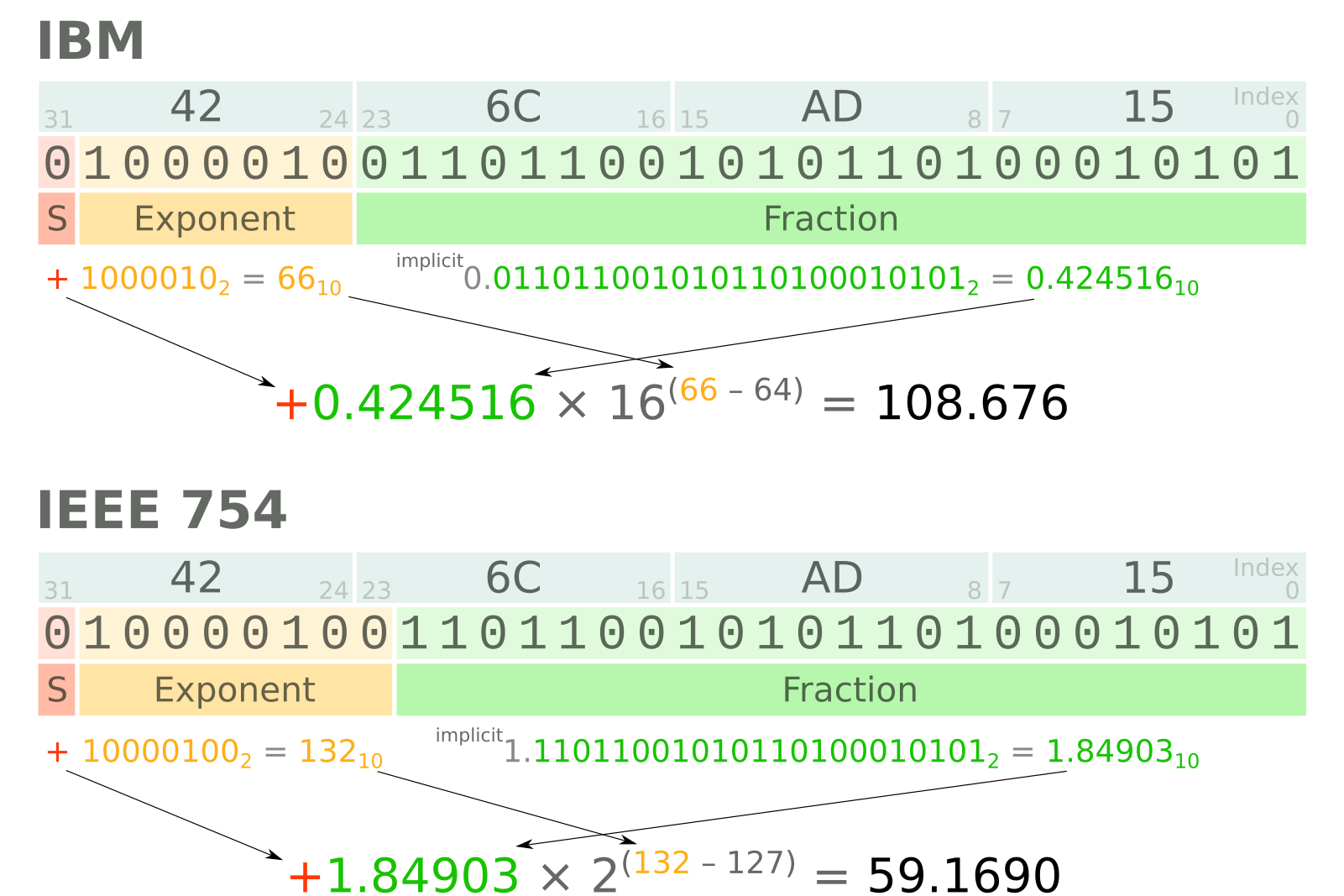
The diagram below shows how four bytes (0x42, 0x6C, 0xAD, 0x15) are interpreted under the two schemes. The results are quite different. Notice the extra bit for the exponent in the IEEE representation, and the different bases and biases.

A four-byte word, 426CAD15 (in hexadecimal), interpreted as an IBM float (top) and an IEEE float (bottom). Most scientists would care about this difference!

A four-byte word, 426CAD15 (in hexadecimal), interpreted as an IBM float (top) and an IEEE float (bottom). Most scientists would care about this difference!

IBM, IEEE, and seismic

When SEG-Y was defined in 1975, there were only IBM floats — IEEE floats were not defined until 1985. The SEG allowed the use of IEEE floating-point numbers in Revision 1 (2002), and they are still allowed in the impending Revision 2 specification. This is important because most computers these days use IEEE float representations, so if you want to read or write IBM floats, you're going to need to do some work.

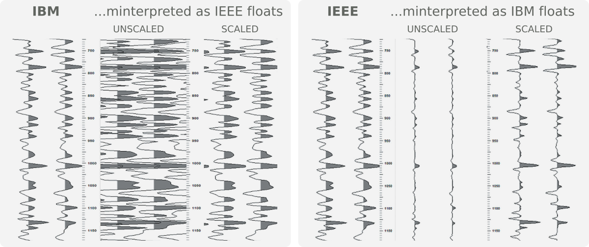
The floating-point format in a particular SEG-Y file should be indicated by a flag in bytes 3225–3226. A value of 0x01 indicates IBM floats, while 0x05 indicates IEEE floats. Then again, you can't believe everything you read in headers. And, unfortunately, you can't tell an IBM float just by looking at it. Meisinger (2004) wrote a nice article in CSEG Recorder about the perils of loading IBM as IEEE and vice versa — illustrated below. You should read it.

From Meisinger, D (2004). SEGY floating point confusion. CSEG Recorder 29(7). Available online.

From Meisinger, D (2004). SEGY floating point confusion. CSEG Recorder 29(7). Available online.

I wrote this post by accident while writing about endianness, the main big change in the new SEG-Y revision. Stay tuned for that post! [Update: here it is!]

The quick green forsterite jumped over the lazy dolomite

The best-known pangram — a sentence containing every letter of the alphabet —  is probably

 
The quick brown fox jumped over the lazy dog.

There are lots of others of course. If you write like James Joyce, there are probably an infinite number of others. The point is to be short, and one of the shortest, with only 29 letters (!), even has a geological flavour:

 
Sphinx of black quartz, judge my vow.

I know what you're thinking: Cool, but what's the shortest set of mineral names that uses all the letters of the alphabet? What logophiliac geologist would not wonder the same thing?

Well, we posed this question in the most recent "Riddle me this" segment on the Undersampled Radio podcast. This blog post is my solution.


The set cover problem

Finding pangrams in a list of words amounts to solving the classical set cover problem:

 
Given a set of elements \(\{U_1, U_2,\ldots , U_n\}\) (called the ‘universe’) and a collection \(S\) of \(m\) sets whose union equals the universe, the set cover problem is to identify the smallest sub-collection of \(S\) whose union equals (or ‘covers’) the universe.

Our universe is the alphabet, and our \(S\) is the list of \(m\) mineral names. There is a slight twist in our case: the set cover problem wants the smallest subset of \(S\) — the fewest members. But in this problem, I suspect there are several 4-word solutions (judging from my experiments), so I want the smallest total size of the members of the subset. That is, I want the fewest total letters in the solution.

The solution

The set cover problem was shown to be NP-complete in 1972. What does this mean? It means that it's easy to tell if you have an answer (do you have all the letters of the alphabet?), but the only way to arrive at a solution is — to oversimplify massively — by brute force. (If you're interested in this stuff, this edition of the BBC's In Our Time is one of the best intros to P vs NP and complexity theory that I know of.)

Anyway, the point is that if we find a better way than brute force to solve this problem, then we need to write a paper about it immediately, claim our prize, collect our turkey, then move to a sunny tax haven with good water and double-digit elevation.

So, this could take a while: there are over 95 billion ways to draw 3 words from my list of 4600 mineral names. If we need 4 minerals, there are 400 trillion combinations... and a quick calculation suggests that my laptop will take a little over 50 years to check all the combinations. 

Can't we speed it up a bit?

Brute force is one thing, but we don't need to be brutish about it. Maybe we can think of some strategies to give ourselves a decent chance:

  • The list is alphabetically sorted, so randomize the list before searching. (I did this.)
  • Guess some 'useful' minerals and ensure that you get to them. (I did this too, with quartz.)
  • Check there are at least 26 letters in the candidate words, and (if it's only records we care about) no more than 44, because I have a solution with 45 letters (see below).
  • We could sort the list into word length order. That way we search shorter things first, so we should get shorter lists (which we want) earlier.
  • My solution does not depend much on Python's set type. Maybe we could do more with set theory.
  • Before inspecting the last word in each list, we could make sure it contains at least one letter that's so far missing.

So far, the best solution I've come up with so far has 45 letters, so there's plenty of room for improvement:

 
'quartz', 'kvanefjeldite', 'abswurmbachite', 'pyroxmangite'

My solution is in this Jupyter Notebook. Please put me out of my misery by improving on it.

SEG machine learning contest: there's still time

Have you been looking for an excuse to find out what machine learning is all about? Or maybe learn a bit of Python programming language? If so, you need to check out Brendon Hall's tutorial in the October issue of The Leading Edge. Entitled, "Facies classification using machine learning", it's a walk-through of a basic statistical learning workflow, applied to a small dataset from the Hugoton gas field in Kansas, USA.

But it was also the launch of a strictly fun contest to see who can get the best prediction from the available data. The rules are spelled out in ther contest's README, but in a nutshell, you can use any reproducible workflow you like in Python, R, Julia or Lua, and you must disclose the complete workflow. The idea is that contestants can learn from each other.

Left: crossplots and histograms of wireline log data, coloured by facies — the idea is to highlight possible data issues, such as highly correlated features. Right: true facies (left) and predicted facies (right) in a validation plot. See the rest of the paper for details.

What's it all about?

The task at hand is to predict sedimentological facies from well logs. Such log-derived facies are sometimes called e-facies. This is a familiar task to many development geoscientists, and there are many, many ways to go about it. In the article, Brendon trains a support vector machine to discriminate between facies. It does a fair job, but the accuracy of the result is less than 50%. The challenge of the contest is to do better.

Indeed, people have already done better; here are the current standings:

Team F1 Algorithm Language Solution
1 gccrowther 0.580 Random forest Python Notebook
2 LA_Team 0.568 DNN Python Notebook
3 gganssle 0.561 DNN Lua Notebook
4 MandMs 0.552 SVM Python Notebook
5 thanish 0.551 Random forest R Notebook
6 geoLEARN 0.530 Random forest Python Notebook
7 CannedGeo 0.512 SVM Python Notebook
8 BrendonHall 0.412 SVM Python Initial score in article

As you can see, DNNs (deep neural networks) are, in keeping with the amazing recent advances in the problem-solving capability of this technology, doing very well on this task. Of the 'shallow' methods, random forests are quite prominent, and indeed are a great first-stop for classification problems as they tend to do quite well with little tuning.

How do I enter?

There is still over 6 weeks to enter: you have until 31 January. There is a little overhead — you need to learn a bit about git and GitHub, there's some programming, and of course machine learning is a massive field to get up to speed on — but don't be discouraged. The very first entry was from Bryan Page, a self-described non-programmer who dusted off some basic skills to improve on Brendon's notebook. But you can run the notebook right here in mybinder.org (if it's up today — it's been a bit flaky lately) and a play around with a few parameters yourself.

The contest aspect is definitely low-key. There's no money on the line — just a goody bag of fun prizes and a shedload of kudos that will surely get the winners into some awesome geophysics parties. My hope is that it will encourage you (yes, you) to have fun playing with data and code, trying to do that magical thing: predict geology from geophysical data.


Reference

Hall, B (2016). Facies classification using machine learning. The Leading Edge 35 (10), 906–909. doi: 10.1190/tle35100906.1. (This paper is open access: you don't have to be an SEG member to read it.)