More ways to make models

A few weeks ago I wrote about a new feature in bruges for making wedge models. This new feature makes it really easy to make wedge models, for example:

 
import bruges as bg import matplotlib.pyplot as plt strat = [(0, 1, 0), (2, 3, 2, 3, 2), (4, 5, 4)] wedge, *_ = bg.models.wedge(strat=strat, conformance=’top’) plt.imshow(wedge)

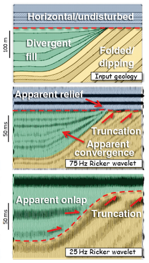
And here are some examples of what this will produce, depending on the conformance argument:
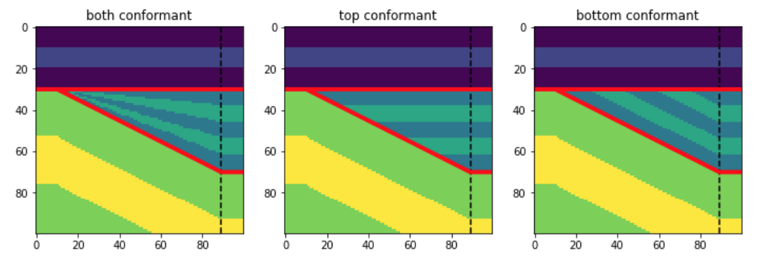
wedge_conformance.png

What’s new

I thought it might be interesting to be able to add another dimension to the wedge model — in and out of the screen in the models shown above. In that new dimension — as long as there are only two rock types in there — we could vary the “net:gross” of the wedge.

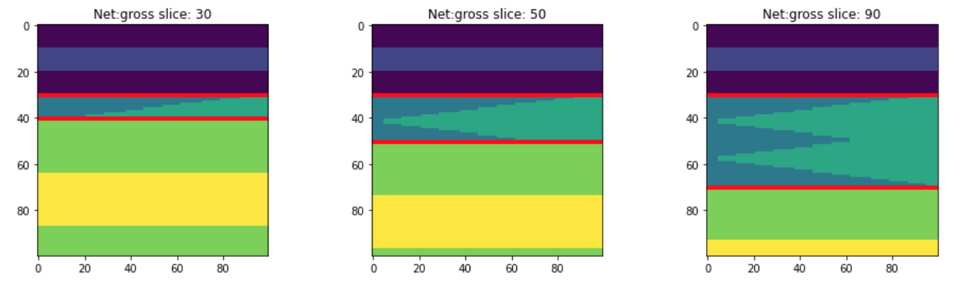
So if we have two rock types in the wedge, let’s say 2 and 3 as in the wedges shown above, we’ll end up with a lot of different wedges. At one end of the new dimension, we’ll have a wedge that is all 2. At the other end, it’ll be all 3. And in between, there’ll be a mixture of 2 and 3, with the layers interfingering in a geometrically symmetric way.

Let’s look at those 3 slices in the central model shown above:

bruges_wedge_slices.png

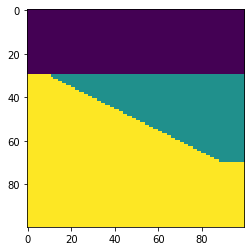
We can also see slices in that other dimension, to visualize the net:gross variance across the model. These slices are near the thin end of the wedge, the middle, and the thick end:

bruges_netgross_slices.png

To get 3D wedge models like this, just make a binary (2-component) wedge and add breadth=100 (the number of slices in the new dimension).

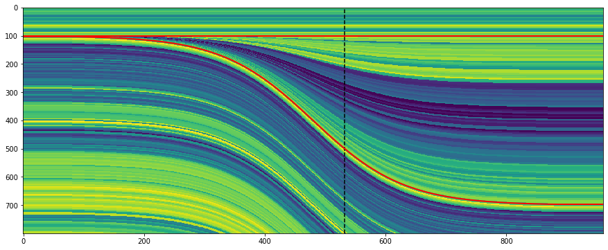
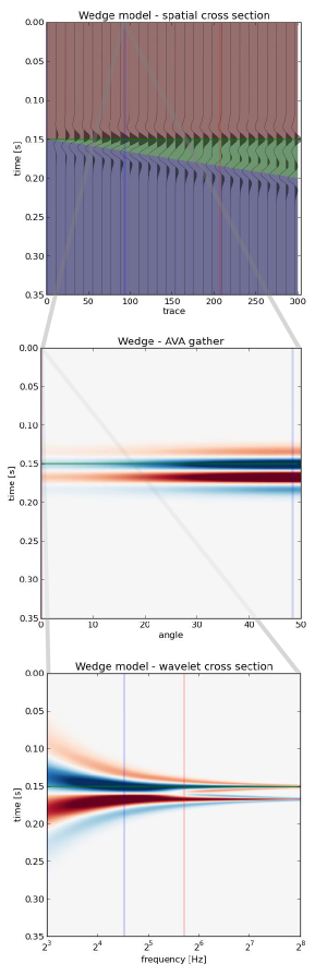
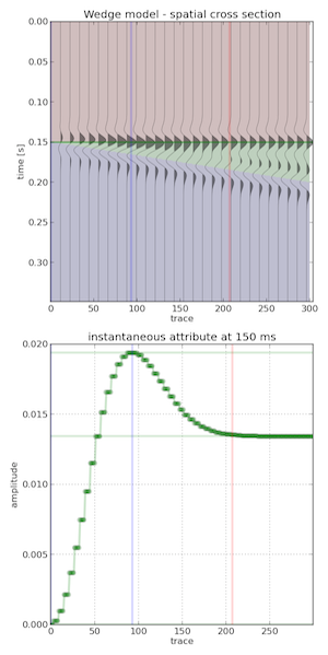
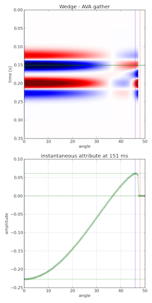
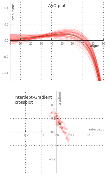
These models are admittedly a little mind-bending. Here’s what slices in all 3 orthogonal directions look like, along with (very badly) simulated seismic through this 3D wedge model:

bruges_all_the_slices.png

New wedge shapes!

As well as the net-to-gross thing, I added some new wedge shapes, so now you can have some steep-sided alternatives to the linear and sigmoidal ramps I had in there originally. In fact, you can pass in a wedge shape function of your own, so there’s no end to what you could implement.

bruges_new_wedge_shapes.png

You can read about these new features in this notebook. Please note that you will need the latest version of bruges to use these new features, so run pip install —upgrade bruges in your environment, then you’ll be all set. Share your models, I’d love to see what you make!

All the wedges

Wedges are a staple of the seismic interpreter’s diet. These simple little models show at a glance how two seismic reflections interact with each other when a rock layer thins down to — and below — the resolution limit of the data. We can also easily study how the interaction changes as we vary the wavelet’s properties, especially its frequency content.

Here’s how to make and plot a basic wedge model with Python in the latest version of bruges, v0.4.2:

 
import bruges as bg
import matplotlib.pyplot as plt

wedge, *_ = bg.models.wedge()

plt.imshow(wedge)
wedge_basic.png

It really is that simple! This model is rather simplistic though: it contains no stratigraphy, and the numerical content of the 2D array is just a bunch of integers. Let’s instead make a P-wave velocity model, with an internal bed of faster rock inside the wedge:

 
strat = [2.35, (2.40, 2.50, 2.40), 2.65]
wedge, *_ = bg.models.wedge(strat=strat)

plt.imshow(wedge)
plt.colorbar()
wedge_layer.png

We can also choose to make the internal geometry top- or bottom-conformant, mimicking onlap or an unconformity, respectively.

 
strat = strat=[0, 7*[1,2], 3]
wedge, *_ = bg.models.wedge(strat=strat,
                            conformance='base'
                           )

plt.imshow(wedge)
wedge_unconformity.png

The killer feature of this new function might be using a log to make the stratigraphy, rather than just a few beds. This is straightforward to do with welly, because it makes selecting depth intervals and resampling a bit easier:

 
import welly

gr = welly.Well.from_las('R-39.las').data['GR']
log_above = gr.to_basis(stop=2620, step=1.0)
log_wedge = gr.to_basis(start=2620, stop=2720, step=1.0)
log_below = gr.to_basis(start=2720, step=1.0)

strat = (log_above, log_wedge, log_below)
depth, width = (100, 400, 100), (40, 200, 40)
wedge, top, base, ref = bg.models.wedge(depth=depth,
                                        width=width,
                                        strat=strat,
                                        thickness=(0, 1.5)
                                       )

plt.figure(figsize=(15, 6))
plt.imshow(wedge, aspect='auto')
plt.axvline(ref, color='k', ls='--')
plt.plot(top, 'r', lw=2)
plt.plot(base, 'r', lw=2)
wedge_log.png

Notice that the function returns to you the top and base of the wedgy part, as well as the position of the ‘reference’, in this case the well.

I’m not sure if anyone wanted this feature… but you can make clinoform models too:

wedge_log_clino.png

Lastly, the whole point of all this was to make a synthetic — the forward model of the seismic experiment. We can make a convolutional model with just a few more lines of code:

 
strat = np.array([2.32 * 2.65,  # Layer 1
                  2.35 * 2.60,  # Layer 2
                  2.35 * 2.62,  # Layer 3
                 ])

# Fancy indexing into the rocks with the model.
wedge, top, base, ref = bg.models.wedge(strat=strat)

# Make reflectivity.
rc = (wedge[1:] - wedge[:-1]) / (wedge[1:] + wedge[:-1])

# Get a wavelet.
ricker = bg.filters.ricker(0.064, 0.001, 40)

# Repeated 1D convolution for a synthetic.
syn = np.apply_along_axis(np.convolve, arr=rc, axis=0, v=ricker, mode='same')
wedge_synthetic.png

That covers most of what the tool can do — for now. I’m working on extending the models to three dimensions, so you will be able to vary layers or rock properties in the 3rd dimension. In the meantime, take these wedges for a spin and see what you can make! Do share your models on Twitter or LinkedIn, and have fun!

x lines of Python: synthetic wedge model

Welcome to a new blog series! Like the A to Z and the Great Geophysicists, I expect it will be sporadic and unpredictable, but I know you enjoys life's little nonlinearities as much as I.

The idea with this one — x lines of Python — is to share small geoscience workflows in x lines or fewer. I'm not sure about the value of x, but I think 10 seems reasonable for most tasks. If x > 10 then the task may have been too big... If x < 5 then it was probably too small.

Python developer Raymond Hettinger says that each line of code should be equivalent to a sentence... so let's say that that's the measure of what's OK to put in a single line. 

Synthetic wedge model

To kick things off, follow this link to a live Jupyter Notebook environment showing how you can make a simple synthetic three-rock wedge model in only 9 lines of code.

The sentences represented by the code that made the data in these images are:

  1. Set up the size of the model.
  2. Make the slanty bit, with 1's in the wedge and 2's in the base.
  3. Add the top of the model as 0; these numbers will turn into rocks.
  4. Define the velocity and density of rocks 0 to 2.
  5. Distribute those properties through the model.
  6. Calculate the acoustic impedance everywhere.
  7. Calculate the reflection coefficients in the model.
  8. Make a Ricker wavelet.
  9. Convolve the wavelet with the reflection coefficients.

Your turn!

All of the notebooks we share in this series will be hosted on mybinder.org. I'm excited about this because it means you can run and edit them live, without installing anything at all. Give it a go right now.

You can see them on GitHub too, and fork or clone them from there. Note that if you look at the notebook for this post on GitHub, you'll be able to view it, but not change or run code unless you get everything running on your own machine. (To do that, you can more or less follow the instructions in my User Guide to the TLE tutorials).

Please do take this notion of x as 'par' as a challenge. If you'd like to try to shoot under par, please do — and share your efforts. Code golf is a fun way to learn better coding habits. (And maybe some bad ones.) There is a good chance I will shoot some bogies on this course.

We will certainly take requests too — what tasks would you like to see in x lines of Python?

A focus on building

We've got some big plans for modelr.io, our online forward modeling tool. They're so big, we're hiring! An exhilarating step for a small company. If you are handy with the JavaScript, or know someone who is, scroll down to read all about it!

Here are some of the cool things in Modelr's roadmap:

Interactive 1D models – to support fluid substitution, we need to handle physical properties of pore fluids as well as rocks. Our prototype (right) supports arbitrary layers, but eventually we'd like to allow uploading well logs too.

Exporting models – imagine creating an earth model of your would-be prospect, and sending it around to your asset team to strengthen it's prognosis. Modelr solves the forward problem, PickThis solves the inverse. We need to link them up. We also need SEG-Y export, so you can see your model next to your real data.

Models from sketches – Want to do a quick sketch of a geologic setting, and see what it would look like under the lens of seismic? At the hackathon last month, Matteo Niccoli and friends showed a path to this dream — sketch a picture, take a photo, and upload it to the the app with your phone (right). 

3D models Want to visualize how seismic amplitudes vary according to bed thickness? Build a 2D wedge model and you can analyze a tuning curve. Now, want to explore the same wedge spanning a range of physical properties? That's a job for a 3D wedge model. 

Seismic attributes – Seismic discontinuity attributes, like continuity, or curvature can be ineffective when viewed in cross-section; they're really meant to be shown in time-slices. There is a vast library of attributes and co-rendering technologies we want to provide.

If you get excited about building simple tools on the web for difficult tasks under the ground, we'd love to talk to you. We have an open position for a full-time web developer to help us carry this project forward. Check out the job posting.

The race for useful offsets

We've been working on a 3D acquisition lately. One of the factors influencing the layout pattern of sources and receivers in a seismic survey is the range of useful offsets over the depth interval of interest. If you've got more than target depth, you'll have more than one range of useful offsets. For shallow targets this range is limited to small offsets, due to direct waves and first breaks. For deeper targets, the range is limited at far offsets by energy losses due to geometric spreading, moveout stretch, and system noise.

In seismic surveying, one must choose a spacing interval between geophones along a receiver line. If phones are spaced close together, we can collect plenty of samples in a small area. If the spacing is far apart, the sample density goes down, but we can collect data over a bigger area. So there is a trade-off and we want to maximize both; high sample density covering the largest possible area.

What are useful offsets?

It isn't immediately intuitive why illuminating shallow targets can be troublesome, but with land seismic surveying in particular, first breaks and near surface refractions clobber shallow reflecting events. In the CMP domain, these are linear signals, used for determining statics, and are discarded by muting them out before migration. Reflections that arrive later than the direct wave and first refractions don't get muted out. But if these reflections arrive later than the air blast noise or ground roll noise — pervasive at near offsets — they get caught up in noise too. This region of the gather isn't muted like the top mute, otherwise you'd remove the data at near offsets. Instead, the gathers are attacked with algorithms to eliminate the noise. The extent of each hyperbola that passes through to migration is what we call the range of useful offsets.

muted_moveout2.png

The deepest reflections have plenty of useful offsets. However if we wanted to do adequate imaging somewhere between the first two reflections, for instance, then we need to make sure that we record redundant ray paths over this smaller range as well. We sometimes call this aperture; the shallow reflection is restricted in the number of offsets that it can be illuminated with, the deeper reflections can tolerate an aperture that is more open. In this image, I'm modelling the case of 60 geophones spanning 3000 metres, spaced evenly at 100 metres apart. This layout suggests merely 4 or 5 ray paths will hit the uppermost reflection, the shortest ray paths at small offsets. Also, there is usually no geophone directly on top of the source location to record a vertical ray path at zero offset. The deepest reflections however, should have plenty of fold, as long as NMO stretch, geometric spreading, and noise levels were good.

The problem with determining the range of useful offsets by way of a model is, not only does it require a velocity profile, which is easily attained from a sonic log, VSP, or velocity analysis, but it also requires an estimation of the the speed, intensity, and duration of the near surface events to be muted. Parameters that depend largely on the nature of the source and the local ground conditions, which vary from place to place, and from one season to the next.

In a future post, we'll apply this notion of useful offsets to build a pattern for shooting a 3D.


Click here for details on how I created this figure using the IPython Notebook. If you don't have it, IPython is easy to install. The easiest way is to install all of scientific Python, or use Canopy or Anaconda.

This post was inspired in part by Norm Cooper's 2004 article, A world of reality: Designing 3D seismic programs for signal, noise, and prestack time-migration. The Leading Edge23 (10), 1007-1014.DOI: 10.1190/1.1813357

Update on 2014-12-17 13:04 by Matt Hall
Don't miss the next installment — Laying out a seismic survey — with more IPython goodness!

Cross sections into seismic sections

We've added to the core functionality of modelr. Instead of creating an arbitrarily shaped wedge (which is plenty useful in its own right), users can now create a synthetic seismogram out of any geology they can think of, or extract from their data.

Turn a geologic-section into an earth model

We implemented a color picker within an image processing scheme, so that each unique colour gets mapped to an editable rock type. Users can create and manage their own rock property catalog, and save models as templates to share and re-use. You can use as many or as few colours as you like, and you'll never run out of rocks.

To give an example, let's use the stratigraphic diagram that Bruce Hart used in making synthetic seismic forward models in his recent Whither seismic stratigraphy article. There are 7 unique colours, so we can generate an earth model by assigning a rock to each of the colours in the image.

If you can imagine it, you can draw it. If you can draw it, you can model it.

Modeling as an interactive experience

We've exposed parameters in the interface and so you can interact with the multidimensional seismic data space. Why is this important? Well, modeling shouldn't be a one-shot deal. It's an iterative process. A feedback cycle where you turn knobs, pull levers, and learn about the behaviour of a physical system; in this case it is the interplay between geologic units and seismic waves. 

A model isn't just a single image, but a swath of possibilities teased out by varying a multitude of inputs. With modelr, the seismic experiment can be manipulated, so that the gamut of geologic variability can be explored. That process is how we train our ability to see geology in seismic.

Hart's paper doesn't specifically mention the rock properties used, so it's difficult to match amplitudes, but you can see here how modelr stands up next to Hart's images for high (75 Hz) and low (25 Hz) frequency Ricker wavelets.

There are some cosmetic differences too... I've used fewer wiggle traces to make it easier to see the seismic waveforms. And I think Bruce forgot the blue strata on his 25 Hz model. But I like this display, with the earth model in the background, and the wiggle traces on top — geology and seismic blended in the same graphical space, as they are in the real world, albeit briefly.


Subscribe to the email list to stay in the loop with modelr news, or sign-up at modelr.io and get started today.

This will add you to the email list for the modeling tool. We never share user details with anyone. You can unsubscribe any time.

Seismic models: Hart, BS (2013). Whither seismic stratigraphy? Interpretation, volume 1 (1). The image is copyright of SEG and AAPG.

Getting started with Modelr

Let's take a closer look at modelr.io, our new modeling tool. Just like real seismic experiments, there are four components:

  • Make a framework. Define the geometries of rock layers.
  • Make an earth. Assign a set of rock properties to each layer.
  • Make a kernel. Define the seismic survey.
  • Make a plot. Set the output parameters.

Modelr takes care of the physics of wave propagation and reflection, so you don't have to stick with normal incidence acoustic impedance models if you don't want to. You can explore the full range of possibilities.

3 ways to slice a wedge

To the uninitiated, the classic 3-layer wedge model may seem ridiculously trivial. Surely the earth looks more complicated than that! But we can leverage such geometric simplicity to systematically study how seismic waveforms change across spatial and non-spatial dimensions. 

Spatial domain. In cross-section (right), a seismic wedge model lets you analyse the resolving power of a given wavelet. In this display the onset of tuning is marked by the vertical red line, and the thickness at which maximum tuning occurs is shown in blue. Reflection profiles can be shown for any incidence angle, or range of incidence angles (offset stack).

Amplitude versus angle (AVA) domain. Maybe you are working on a seismic inversion problem so you might want to see what a CDP angle gather looks like above and below tuning thickness. Will a tuned AVA response change your quantitative analysis? This 3-layer model looks like a two-layer AVA gather except our original wavelet looks like it has undergone a 90 degree phase rotation. Looks can be deceiving. 

Amplitude versus frequency domain. If you are trying to design a seismic source for your next survey, and you want to ensure you've got sufficient bandwidth to resolve a thin bed, you can compute a frequency gather — right, bottom — and explore a swath of wavelets with regard to critical thickness in your prospect. The tuning frequency (blue) and resolving frequency (red) are revealed in this domain as well. 

Wedges are tools for seismic waveform classification. We aren't just interested in digitizing peaks and troughs, but the subtle interplay of amplitude tuning, and apparent phase rotation variations across the range of angles and bandwidths in the seismic experiment. We need to know what we can expect from the data, from our supposed geology. 

In a nutshell, all seismic models are about illustrating the band-limited nature of seismic data on specific geologic scenarios. They help us calibrate our intuition when bandwidth causes ambiguity in interpretation. Which is nearly all of the time.

Calibrate your seismic intuition

On Tuesday we announced our new web app, modelr.io. Why are we so excited about it? 

  • We love the idea that subsurface software can cost dollars, not 1000's of dollars. 
  • We love the idea of subsurface software being online, not on the desktop.
  • We love the idea that subsurface software can be open source. Here's our code!
  • We love the idea of subsurface software that doesn't need a manual to master.
  • We love the idea of subsurface software that runs on a tablet or a phone.
  • We see software as an important way to share knowledge and connect people.

OK, that's enough reasons. There are more. Those are the main ones.

The point is: we love these ideas. And we hope that you, dear reader, at least like some of them a bit. Because we really want to keep developing modelr. We think it can be awesome. Imagine 3D earth models, imagine full waveform modeling, imagine gravity and magnetic models. We get very excited when we think about all the possiblities. There's no better way to calibrate your seismic intuition than modeling, and modelr is a great place to start modeling. 

Here's a challenge: take 3 minutes and see if you can generate...

 A wedge model & tuning curve An AVA gather for a Class 4 sand    A stochastic AVA crossplot          

 modelr seismic wedge modelmodelr seismic avo modelmodelr stochastic avo  model

The most important thing nobody does

A couple of weeks ago, we told you we were up to something. Today, we're excited to announce modelr.io — a new seismic forward modeling tool for interpreters and the seismically inclined.

Modelr is a web app, so it runs in the browser, on any device. You don't need permission to try it, and there's never anything to install. No licenses, no dongles, no not being able to run it at home, or on the train.

Later this week, we'll look at some of the things Modelr can do. In the meantime, please have a play with it.
Just go to modelr.io and hit Demo, or click on the screenshot below. If you like what you see, then think about signing up — the more support we get, the faster we can make it into the awesome tool we believe it can be. And tell your friends!

If you're intrigued but unconvinced, sign up for occasional news about Modelr:

This will add you to the email list for the modeling tool. We never share user details with anyone. You can unsubscribe any time.

Transforming geology into seismic

Hart (2013). ©SEG/AAPGForward modeling of seismic data is the most important workflow that nobody does.

Why is it important?

  • Communicate with your team. You know your seismic has a peak frequency of 22 Hz and your target is 15–50 m thick. Modeling can help illustrate the likely resolution limits of your data, and how much better it would be with twice the bandwidth, or half the noise.
  • Calibrate your attributes. Sure, the wells are wet, but what if they had gas in that thick sand? You can predict the effects of changing the lithology, or thickness, or porosity, or anything else, on your seismic data.
  • Calibrate your intuition. Only by predicting the seismic reponse of the geology you think you're dealing with, and comparing this with the response you actually get, can you start to get a feel for what you're really interpreting. Viz Bruce Hart's great review paper we mentioned last year (right).

Why does nobody do it?

Well, not 'nobody'. Most interpreters make 1D forward models — synthetic seismograms — as part of the well tie workflow. Model gathers are common in AVO analysis. But it's very unusual to see other 2D models, and I'm not sure I've ever seen a 3D model outside of an academic environment. Why is this, when there's so much to be gained? I don't know, but I think it has something to do with software.

  • Subsurface software is niche. So vendors are looking at a small group of users for almost any workflow, let alone one that nobody does. So the market isn't very competitive.
  • Modeling workflows aren't rocket surgery, but they are a bit tricky. There's geology, there's signal processing, there's big equations, there's rock physics. Not to mention data wrangling. Who's up for that?
  • Big companies tend to buy one or two licenses of niche software, because it tends to be expensive and there are software committees and gatekeepers to negotiate with. So no-one who needs it has access to it. So you give up and go back to drawing wedges and wavelets in PowerPoint.

Okay, I get it, how is this helping?

We've been busy lately building something we hope will help. We're really, really excited about it. It's on the web, so it runs on any device. It doesn't cost thousands of dollars. And it makes forward models...

That's all I'm saying for now. To be the first to hear when it's out, sign up for news here:

This will add you to the email list for the modeling tool. We never share user details with anyone. You can unsubscribe any time.

Seismic models: Hart, BS (2013). Whither seismic stratigraphy? Interpretation, volume 1 (1). The image is copyright of SEG and AAPG.