Geoscientist, challenge thyself

No costume is required for solving geocomputing kata

One of the highlights of my year is the Advent of Code, a sort of advent calendar for nerds. Its creator, Eric Wastl (hear his story), releases a new puzzle every day from the 1st of the month up to Christmas day. And the productivity of the global developer community goes down 74%.

Ever since the first one I tried, I’ve been wondering what geological coding challenges might look like. And now, 18 months later… well, I still don’t know, but I’ve made some anyway!

Puzzle number 1 (or 0)

Here’s how the first one starts:

You have a string of lithology codes, reading from the bottom up of a geological section. There is a sample every metre. There are three lithologies:

• Mudstone
• Fine sandstone or siltstone
• Sandstone

The strings look like this:

    ...MFFSSFSSSS...

Your data, when you receive it, will be much longer than this.

We need to get some geological information from this string of codes. Specifically, you need to answer 3 questions:

1. What is the total thickess in metres of sandstone (S)? Each sample represents one metre.
2. How many sandstone beds are there? A bed is a contiguous group of one lithology, so MMFFF is 2 beds, one of M and one of F.
3. How many times does the most common upwards bed transition occur? Do not include transitions from a lithology to itself.

You can download your own personal dataset, which in this case has 20,000 lithology codes. Then you can try to answer the questions, one at a time. You can use any programming language — indeed, any method at all — to solve the problems, you give an answer back to the server, and it will tell you if you are correct or not.

There are, as of right now, five ‘chapters’, covering topics from naming rock samples to combining map layers. You will receive the name of the next chapter when you correctly answer the final question of the three or four in each challenge.

If you’d like to give it a try, there’s a live starter Jupyter notebook here:

https://ageo.co/kata-live

Or, if you prefer, there’s a static notebook at https://ageo.co/kata, or you can dive directly into the web API for the first challenge: https://kata.geosci.ai/challenge/sequence

Do let us know how you get on!

The quick green forsterite jumped over the lazy dolomite

The best-known pangram — a sentence containing every letter of the alphabet —  is probably

“The quick brown fox jumped over the lazy dog.”

There are lots of others of course. If you write like James Joyce, there are probably an infinite number of others. The point is to be short, and one of the shortest, with only 29 letters (!), even has a geological flavour:

“Sphinx of black quartz, judge my vow.”

I know what you're thinking: Cool, but what's the shortest set of mineral names that uses all the letters of the alphabet? What logophiliac geologist would not wonder the same thing?

Well, we posed this question in the most recent "Riddle me this" segment on the Undersampled Radio podcast. This blog post is my solution.

---

The set cover problem

Finding pangrams in a list of words amounts to solving the classical set cover problem:

“Given a set of elements \(\{U_1, U_2,\ldots , U_n\}\) (called the ‘universe’) and a collection \(S\) of \(m\) sets whose union equals the universe, the set cover problem is to identify the smallest sub-collection of \(S\) whose union equals (or ‘covers’) the universe.”

Our universe is the alphabet, and our \(S\) is the list of \(m\) mineral names. There is a slight twist in our case: the set cover problem wants the smallest subset of \(S\) — the fewest members. But in this problem, I suspect there are several 4-word solutions (judging from my experiments), so I want the smallest total size of the members of the subset. That is, I want the fewest total letters in the solution.

The solution

The set cover problem was shown to be NP-complete in 1972. What does this mean? It means that it's easy to tell if you have an answer (do you have all the letters of the alphabet?), but the only way to arrive at a solution is — to oversimplify massively — by brute force. (If you're interested in this stuff, this edition of the BBC's In Our Time is one of the best intros to P vs NP and complexity theory that I know of.)

Anyway, the point is that if we find a better way than brute force to solve this problem, then we need to write a paper about it immediately, claim our prize, collect our turkey, then move to a sunny tax haven with good water and double-digit elevation.

So, this could take a while: there are over 95 billion ways to draw 3 words from my list of 4600 mineral names. If we need 4 minerals, there are 400 trillion combinations... and a quick calculation suggests that my laptop will take a little over 50 years to check all the combinations. 

Can't we speed it up a bit?

Brute force is one thing, but we don't need to be brutish about it. Maybe we can think of some strategies to give ourselves a decent chance:

• The list is alphabetically sorted, so randomize the list before searching. (I did this.)
• Guess some 'useful' minerals and ensure that you get to them. (I did this too, with quartz.)
• Check there are at least 26 letters in the candidate words, and (if it's only records we care about) no more than 44, because I have a solution with 45 letters (see below).
• We could sort the list into word length order. That way we search shorter things first, so we should get shorter lists (which we want) earlier.
• My solution does not depend much on Python's set type. Maybe we could do more with set theory.
• Before inspecting the last word in each list, we could make sure it contains at least one letter that's so far missing.

So far, the best solution I've come up with so far has 45 letters, so there's plenty of room for improvement:

'quartz', 'kvanefjeldite', 'abswurmbachite', 'pyroxmangite'

My solution is in this Jupyter Notebook. Please put me out of my misery by improving on it.

Reliable predictions of unlikely geology

A puzzle

Imagine you are working in a newly-accessible and under-explored area of an otherwise mature basin. Statistics show that on average 10% of structures are filled with gas; the rest are dry. Fortunately, you have some seismic analysis technology that allows you to predict the presence of gas with 80% reliability. In other words, four out of five gas-filled structures test positive with the technique, and when it is applied to water-filled structures, it gives a negative result four times out of five.

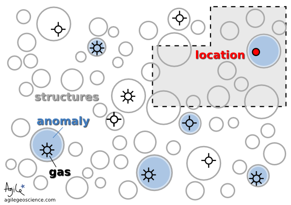
← It is thought that 10% of the structures in this play are gas-filled. Your seismic attribute test is thought to be 80% reliable, because four out of five times it has indicated gas correctly. You acquire the undrilled acreage shown by the grey polygon.

You acquire some undrilled acreage—the grey polygon— then delineate some structures and perform the analysis. One of the structures tests positive. If this is the only information you have, what is the probability that it is gas-filled?

This is a classic problem of embracing Bayesian likelihood and ignoring your built-in 'representativeness heuristic' (Kahneman et al, 1982, Judgment Under Uncertainty: Heuristics and Biases, Cambridge University Press). Bayesian probability combination does not come very naturally to most people but, once understood, can at least help you see the way to approach similar problems in the future. The way the problem is framed here, it is identical to the original formulation of Kahneman et al, the Taxicab Problem. This takes place in a town with 90 yellow cabs and 10 blue ones. A taxi is involved in a hit-and-run, witnessed by a passer-by. Eye witness reliability is shown to be 80%, so if the witness says the taxi was blue, what is the probability that the cab was indeed blue? Most people go with 80%, but in fact the witness is probably wrong. To see why, let's go back to the exploration problem and look at 100 test cases.

Break it down

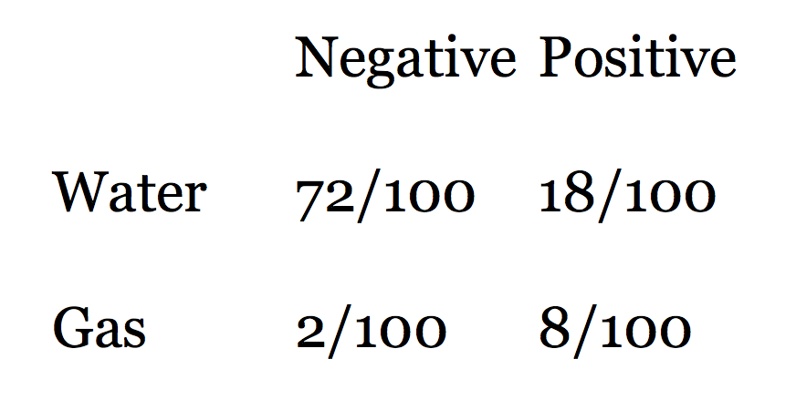
Looking at the rows in this table of outcomes, we see that there are 90 water cases and 10 gas cases. Eighty percent of the water cases test negative, and 80% of the gas cases test positive. The table shows that when we get a positive test, the probability that the test is true is not 0.80, but much less: 8/(8+18) = 0.31. In other words, a test that is mostly reliable is probably wrong when applied to an event that doesn't happen very often (a structure being gas charged). It's still good news for us, though, because a probability of discovery of 0.31 is much better than the 0.10 that we started with.

Here is Bayes' Theorem for calculating the probability P of event A (say, a gas discovery) given event B (say, a positive test in our seismic analysis):

So we can express our problem in these terms:

Are you sure about that?

This result is so counter-intuitive, for me at least, that I can't resist illustrating it with another well-known example that takes it to extremes. Imagine you test positive for a very rare disease, seismitis. The test is 99% reliable. But the disease affects only 1 person in 10 000. What is the probability that you do indeed have seismitis?

Notice that the unreliability (1%) of the test is much greater than the rate of occurrence of the disease (0.01%). This is a red flag. It's not hard to see that there will be many false positives: only 1 person in 10 000 are ill, and that person tests positive 99% of the time (almost always). The problem is that 1% of the 9 999 healthy people, 100 people, will test positive too. So for every 10 000 people tested, 101 test positive even though only 1 is ill. So the probability of being ill, given a positive test, is only about 1/101!

Lessons learned

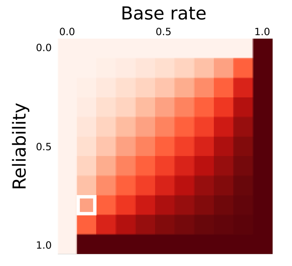
← Predictive power (in Bayesian jargon, the posterior probability) as a function of test reliability and the base rate of occurrence (also called the prior probability of the event of phenomenon in question). The position of the scenario in the exploration problem is shown by the white square.

Thanks to UBC Bioinformatics for the heatmap software, heatmap.notlong.com.

Next time you confidently predict something with a seismic attribute, stop to think not only about the reliability of the test you have made, but the rate of occurrence of the thing you're trying to predict. The heatmap shows how prediction power depends on both test reliability and the occurrence rate of the event. You may be doing worse (or better!) than you think.

Fortunately, in most real cases, there is a simple mitigation: use other, independent, methods of prediction. Mutually uncorrelated seismic attributes, well data, engineering test results, if applied diligently, can improve the odds of a correct prediction. But computing the posterior probability of event A given independent observations B, C, D, E, and F, is beyond the scope of this article (not to mention this author!).

This post is a version of part of my article The rational geoscientist, The Leading Edge, May 2010

Update on 2011-07-12 23:31 by Matt Hall

Just flicking through the archives and came across this post about unlikely events and Bayes' theorem. I can't believe I forgot to link to it in this story. So I'm doing it now!

Confounded paradox

Probabilities are notoriously slippery things to deal with, so it shouldn’t be surprising that proportions, which are really probabilities in disguise, can catch us out too.

Simpson’s paradox is my favourite example of something simple, something we know we understand, indeed have always understood, suddenly turning on us.

Exploration geophysicists often use information extracted from seismic data, called attributes, to help predict rock properties in the subsurface. Suppose you are a geophysicist comparing two new seismic attributes, truth and beauty, each purported to predict fluid type. You compare their hydrocarbon-predicting success rates on 35 discoveries and it’s close, but beauty has an 83% hit rate, while truth manages only 77%. There's not much in it, but since you only need one attribute, all else being equal, beauty it is.

But then someone asks you about predicting oil in particular. You dig out your data and drill down:

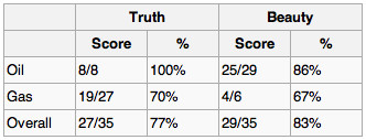
Apparently, truth did a little better when you just look at oil. And what about gas, they ask? Well, the data showed that truth was also better than beauty at predicting gas. So truth does a better job at both oil and gas, but somehow beauty edges out overall.

Impossible? Clearly not: these numbers are real and plausible, I haven't done anything sneaky. In this case, hydrocarbon type is a confounding variable, and it’s important to look for such groupings in your data. Improbable? No, it’s quite common in all kinds of data and this trap is well known among statisticians.

How can you avoid it? Be especially wary when the sample size in one or more of the groups you are interested in is much smaller than the others. Be even more alert if group sizes are inconsistent across the variables, as in my example: oil is under-sampled for truth, gas for beauty.

Ultimately, there's no guarantee this effect won’t crop up; that’s just how proportions are. All you can do is make sure you ask your data the questions you care about. 

This post is a version of part of my article The rational geoscientist, The Leading Edge, May 2010