Backwards and forwards reasoning

Most people, if you describe a train of events to them will tell you what the result will be. There will be few people however, that if you told them a result, would be able to evolve from their own consciousness what the steps were that led to that result. This is what I mean when I talk about reasoning backward.

— Sherlock Holmes, A Study in Scarlet, Sir Arthur Conan Doyle (1887)

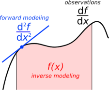
Reasoning backwards is the process of solving an inverse problem — estimating a physical system from indirect data. Straight-up reasoning, which we call the forward problem, is a kind of data collection: empiricism. It obeys a natural causality by which we relate model parameters to the data that we observe.

Modeling a measurement

Where are you headed? Every subsurface problem can be expressed as the arrow between two or more such panels.Inverse problems exists for two reasons. We are incapable of measuring what we are actually interested in, and it is impossible to measure a subject in enough detail, and in all aspects that matter. If, for instance, I ask you to determine my weight, you will be troubled if the only tool I allow is a ruler. Even if you are incredibly accurate with your tool, at best, you can construct only an estimation of the desired quantity. This estimation of reality is what we call a model. The process of estimation is called inversion.

Measuring a model

Forward problems are ways in which we acquire information about natural phenomena. Given a model (me, say), it is easy to measure some property (my height, say) accurately and precisely. But given my height as the starting point, it is impossible to estimate the me from which it came. This is an example of an ill-posed problem. In this case, there is an infinite number of models that share my measurements, though each model is described by one exact solution. 

Solving forward problems are nessecary to determine if a model fits a set of observations. So you'd expect it to be performed as a routine compliment to interpretation; a way to validate our assumptions, and train our intuition.  

The math of reasoning

Forward and inverse problems can be cast in this seemingly simple equation.

where d is a vector containing N observations (the data), m is a vector of M model parameters (the model), and G is a N × M matrix operator that connects the two. The structure of G changes depending on the problem, but it is where 'the experiment' goes. Given a set of model parameters m, the forward problem is to predict the data d produced by the experiment. This is as simple as plugging values into a system of equations. The inverse problem is much more difficult: given a set of observations d, estimate the model parameters m.

I think interpreters should describe their work within the Gm = d framework. Doing so would safeguard against mixing up observations, which should be objective, and interpretations, which contain assumptions. Know the difference between m and d. Express it with an arrow on a diagram if you like, to make it clear which direction you are heading in.

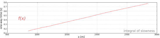
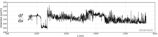
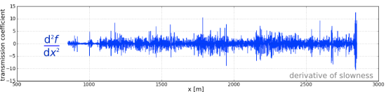
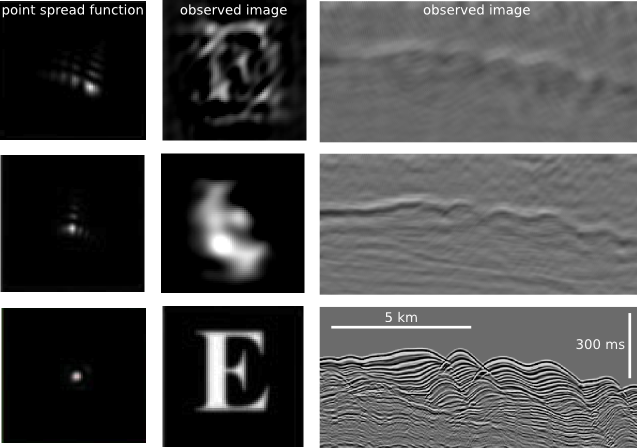
Illustrations for this post were created using data from the Marmousi synthetic seismic data set. The blue seismic trace and its corresponding velocity profile is at location no. 250.

How to get paid big bucks

Yesterday I asked 'What is inversion?' and started looking at problems in geoscience as either forward problems or inverse problems. So what are some examples of inverse problems in geoscience? Reversing our forward problem examples:

• Given a suite of sedimentological observations, provide the depositional environment. This is a hard problem, because different environments can produce similar-looking facies. It is ill-conditioned, because small changes in the input (e.g. the presence of glaucony, or Cylindrichnus) produces large changes in the interpretation.
• Given a seismic trace, produce an impedance log. Without a wavelet, we cannot uniquely deduce the impedance log — there are infinitely many combinations of log and wavelet that will give rise to the same seismic trace. This is the challenge of seismic inversion. 

To solve these problems, we must use induction — a fancy name for informed guesswork. For example, we can use judgement about likely wavelets, or the expected geology, to constrain the geophysical problem and reduce the number of possibilities. This, as they say, is why we're paid the big bucks. Indeed, perhaps we can generalize: people who are paid big bucks are solving inverse problems...

• How do we balance the budget?
• What combination of chemicals might cure pancreatic cancer?
• What musical score would best complement this screenplay?
• How do I act to portray a grief-stricken war veteran who loves ballet?

What was the last inverse problem you solved?

Update on 2013-04-17 21:50 by Matt Hall

Moar inversion! Don't miss the previous post in this mini-series, or the next one — where things get a bit more mathy. 

What is inversion?

Inverse problems are at the heart of geoscience. But I only hear hardcore geophysicists talk about them. Maybe this is because they're hard problems to solve, requiring mathematical rigour and computational clout. But the language is useful, and the realization that some problems are just damn hard — unsolvable, even — is actually kind of liberating. 

Forwards first

Before worrying about inverse problems, it helps to understand what a forward problem is. A forward problem starts with plenty of inputs, and asks for a straightforward, algorithmic, computable output. For example:

• What is 4 × 5?
• Given a depositional environment, what sedimentological features do we expect?
• Given an impedance log and a wavelet, compute a synthetic seismogram.

These problems are solved by deductive reasoning, and have outcomes that are no less certain than the inputs.

Can you do it backwards?

You can guess what an inverse problem looks like. Computing 4 × 5 was pretty easy, even for a geophysicist, but it's not only difficult to do it backwards, it's impossible:

20 = what × what

You can solve it easily enough, but solutions are, to use the jargon, non-unique: 2 × 10, 7.2 × 1.666..., 6.3662 × π — you get the idea. One way to deal with such under-determined systems of equations is to know about, or guess, some constraints. For example, perhaps our system — our model — only includes integers. That narrows it down to three solutions. If we also know that the integers are less than 10, there can be only one solution.

Non-uniqueness is a characteristic of ill-posed problems. Ill-posedness is a dead giveaway of an inverse problem. Proposed by Jacques Hadamard, the concept is the opposite of well-posedness, which has three criteria:

• A solution exists.
• The solution is unique.
• The solution is well-conditioned, which means it doesn't change disproportionately when the input changes. 

Notice the way the example problem was presented: one equation, two unknowns. There is already a priori knowledge about the system: there are two numbers, and the operator is multiplication. In geoscience, since the earth is not a computer, we depend on such knowledge about the nature of the system — what the variables are, how they interact, etc. We are always working with a model of nature.

Tomorrow, I'll look at some specific examples of inverse problems, and Evan will continue the conversation next week.

Update on 2013-04-12 11:18 by Matt Hall

Don't miss the first follow-up to this article, How to get paid big bucks. 

The calculus of geology

Calculus is the tool for studying things that change. Even so, in the midst of the dynamic and heterogeneous earth, calculus is an under-practised and, around the water-cooler at least, under-celebrated workhorse. Maybe that's because people don't realize it's all around us. Let's change that. 

Derivatives of duration

We can plot the time f(x) that passes as a seismic wave travels though space x. This function is known to many geophysicists as the time-to-depth function. It is key for converting borehole measurements, effectively recorded using a measuring tape, to seismic measurements, recorded using a stop watch.

Now let's take the derivative of f(x) with repsect to x. The result is the slowness function (the reciprocal of interval velocity):

The time duration that a seismic wave travels over a small interval (one metre). This function is an actual sonic well log. Differentiating once again yields this curious spiky function:

Geophysicists will spot that this resembles a reflection coefficient series, which governs seismic amplitudes. This is actually a transmission coefficient function, but that small detail is beside the point. In this example, the creating a synthetic seismogram mimics the calculus of geology. 

If you are familiar with the integrated trace attribute, you will recognize that it is an attempt to compute geology by integrating reflectivity spikes. The only issue in this case, and it is a major issue, is that the seismic trace is bandlimited. It does not contain all the information about the earth's slowness. So the earth's geology remains elusive and blurry.

The derivative of slowness yields the reflection boundaries, the integral of slowness yields their position. So in geophysics speak, I wonder, is forward modeling akin to differentiation, and inverse modeling akin to integration? I find it fascinating that these three functions have essentially the same density of information, yet they look increasingly complicated when we take derivatives. 

What other functions do you come across that might benefit from the calculus treatment?

The sonic log used in this example is from the O-32-B/11-E-64 well onshore Nova Scotia, which is publically available but not easily accessible online.

Review: The Wave Watcher's Companion

Visit Amazon.com

The Wave Watcher's Companion: From Ocean Waves to Light Waves via Shock Waves, Stadium Waves, and All the Rest of Life's Undulations
Gavin Pretor-Pinney, Perigee (USA), Bloomsbury (UK), July 2010, $22.95

This book was on my reading list, and then on my shelf, for ages. Now I wish I'd snapped it up and read it immediately. In my defence, the end of 2010 was a busy time for me, what with turning my career upside down and everything, but I'm sure there's a lesson there somewhere...

If you think of yourself as a geophysicist, stop reading this review and buy this book immediately. 

OK, now they've gone, we can look more closely. Gavin Pretor-Pinney is the chap behind The Cloud Appreciation Society, the author of The Cloudspotter's Guide, and co-creator of The Idler Magazine. He not a scientist, but a witty writer with a high curiosity index. The book reads like an extended blog post, or a chat in the pub. A really geeky chat. 

Geophysicists are naturally drawn to all things wavy, but the book touches on sedimentology too — from dunes to tsunamis to seiches. Indeed, the author prods at some interesting questions about what exactly waves are, and whether bedforms like dunes (right) qualify as waves or not. According to Andreas Baas, "it all depends on how loose is your definition of a wave." Pretor-Pinney likes to connect all possible dots, so he settles for a loose definition, backing it up with comparisons to tanks and traffic jams. 

The most eye-opening part for me was Chapter 6, The Fifth Wave, about shock waves. I never knew that there's a whole class of waves that don't obey the normal rules of wave motion: they don't obey the speed limits, they don't reflect or refract properly, and they can't even be bothered to interfere like normal (that is, linear) waves. Just one of those moments when you realize that everything you think you know is actually a gross simplification. I love those moments.

The book is a little light on explanation. Quite a few of the more interesting parts end a little abruptly with something like, "weird, huh?". But there are plenty of notes for keeners to follow up on, and the upside is the jaunty pace and adventurous mix of examples. This one goes on my 're-read some day' shelf. (I don't re-read books, but it's the thought that counts).

Figure excerpt from Pretor-Pinney's book, copyright of the author and Penguin Publishing USA. Considered fair use.

Interpreting spectral gamma-ray logs

Before you can start interpreting spectral gamma-ray logs (or, indeed, any kind of data), you need to ask about quality.

Calibrate your tool...

The main issues affecting the quality of the logs are tool calibration and drilling mud composition. I think there's a tendency to assume that delivered logs have been rigorously quality checked, but... they haven't. The only safe assumption is that nobody cares about your logs as much as you. (There is a huge opportunity for service companies here — but in my experience they tend to be focused on speed and quantity, not quality.)

Calibration is critical. The measurement device in the tool consists of a thallium-laced NaI crystal and a photomultiplier. Both of these components are sensitive to temperature, so calibration is especially important when the temperature of the tool is changing often. If the surface temperature is very different from the downhole—winter in Canada—calibrate often.

Drilling mud containing KCl (to improve borehole stability) increases the apparent potassium content of the formation, while barite acts as a gamma-ray absorber and reduces the count rates, especially in the low energies (potassium).

One of the key quality control indicators is negative readings on the uranium log. A few negative values are normal, but many zero-crossings may indicate that the tool was improperly calibrated. It is imperative to quality control all of the logs, for bad readings and pick-up effects, before doing any quantitative work.

...and your interpretation

Most interpretations of spectral-gamma ray logs focus on the relationships between the three elemental concentrations. In particular, Th/K and Th/U are often used for petrophysical interpretation and log correlation. In calculating these ratios, Schlumberger uses the following cut-offs: if uranium < 0.5 then uranium = 0.5; if potassium < 0.004 then potassium = 0.001 (according to my reference manual for the natural gamma tool).

In general, high K values may be caused by the presence of potassium feldspars or micas. Glauconite usually produces a spike in the K log. High Th values may be associated with the presence of heavy minerals, particularly in channel deposits. Increased Th values may also be associated with an increased input of terrigenous clays. Increases in U are frequently associated with the presence of organic matter. For example, according to the ODP, particularly high U concentrations (> 5 ppm) and low Th/U ratios (< 2) often occur in black shale deposits.

The logs here, from Kansas Geological Survey open file 90-27 by Macfarlane et al. shows a quite overt interpretive approach, with the Th/K log labelled with minerals (feldspar, mica, illite–smectite) and the Th/U log in uranium 'fixedness', a proxy for organic matter.

Sounds useful. But really, you can probably find just a paper to support just about any interpretation you want to make. Which isn't to say that spectral gamma-ray is no use — it's just not diagnostic on its own. You need to calibrate it to your own basin and your own stratigraphy. This means careful, preferably quantitative, comparison of core and logs. 

Further reading 

• Ross Crain's Petrophysical Handbook is a mine of well logging goodness
• Paul Glover's MSc course notes are very comprehensive on most well logging topics
• Fabricius et al. (2003). Geological Survey of Denmark and Greenland Bulletin 1, 349–366. A case stuudy from the Danish Central Graben. 

What is spectral gamma-ray?

The spectral gamma-ray log is a measure of the natural radiation in rocks. The amplitude of the signal from the gamma-ray tool, which is just a sensor with no active source, is proportional to the energy of the gamma-ray photons it encounters. Being able to differentiate between photons of different energies turns out to be very handy Compared to the ordinary gamma-ray log, which ignores the energies and only counts the photons, it's like seeing in colour instead of black and white.

Why do we care about gamma radiation?

First, what are gamma rays? Highly energetic photons: electromagnetic radiation with very short wavelengths. 

Being able to see different energies, or 'colours', means we can differentiate between the radioactive decay of different elements. Elements decay by radiating energy, and the 'colour' of that energy is characteristic of that element (actually, of each isotope). So, we can tell by looking at the energy of a photon if we are seeing a potassium atom (⁴⁰K) or a uranium atom (²³⁸U) decay. These are very different isotopes, with very different habits. We can do geology!

In fact, all sorts of radioisotopes occur naturally in the earth. By far the most abundant are potassium ⁴⁰K, thorium ²³²Th and uranium ²³⁸U. Of these, potassium is the most abundant in sedimentary rocks, but thorium and uranium are present in small quantities, and have particular sedimentological implications.

What exactly are we measuring?

Potassium ⁴⁰K decays to argon about 10% of the time, with γ-emission at 1.46 MeV (the other 90% of the time it decays to calcium). However, all of the decay in the ²³²Th and ²³⁸U decay series occurs by α- and β-particle decay, which don't always result in photon emission. The tool in fact measures γ-radiation from the decay of thallium ²⁰⁸Tl in the ²³²Th series (right), and from bismuth ²¹⁴Bi in the ²³⁸U series. The spectral gamma-ray tool must be calibrated to known samples to give concentrations of ²³²Th and ²³⁸U from its readings. Proper calibration is vital, and is temperature-sensitive (of note in Canada!).

The concentrations of the three elements are estimated from the spectral measure­ments. The concentration of potassium is usually measured in percent (%) or per mil (‰), or sometimes in kilograms per tonne, which is equivalent to per mil. The other two elements are measured in parts per million (ppm).

Here is the gamma-ray spectrum from a single sample from 509 m below the sea-floor at ODP Site 1201. The final spectrum (heavy black line) is shown after removing the background spectrum (gray region) and applying a three-point mean boxcar filter. The thin black line shows the raw spectrum. Vertical lines mark the interval boundaries defined by Peter Blum (an ODP scientist at Texas A&M). Prominent energy peaks relating to certain elements are identified at the top of the figure. The inset shows the spectrum for energies >1500 keV at an expanded scale. 

We wouldn't normally look at these spectra. Instead, the tool provides logs for K, Th, and U. Next time, I'll look at the logs.

Spectrum illustration by Wikipedia user Inductiveload, licensed GFDL; decay chain by Wikipedia user BatesIsBack, licensed CC-BY-SA.

Making images or making prospects?

Well-rounded geophysicists will have experience in each of the following three areas: acquisition, processing, and interpretation. Generally speaking, these three areas make up the seismic method, each requiring highly specified knowledge and tools. Historically, energy companies used to control the entire spectrum, owning the technology, the know-how and the risk, but that is no longer the case. Now, service companies do the acquisition and the processing. Interpretation is largely hosted within E & P companies, the ones who buy land and drill wells. Not only has it become unreasonable for a single geophysicist to be proficient across the board, but organizational structures constrain any particular technical viewpoint. 

Aligning with the industry's strategy, if you are a geophysicist, you likely fall into one of two camps: those who make images, or those who make prospects. One set of people to make the data, one set of people to do the interpretation.

This seems very un-scientific to me.

Where does science fit in?

Science, the standard approach of rational inquiry and accruing knowledge, is largely vacant from the applied geophysical business landscape. But, when science is used as a model, making images and making prospects are inseperable.

Can applied geophysics use scientific behaviour as a central anchor across disciplines?

There is a significant amount of science that is needed in the way that we produce observations, in the way that we make images. But the business landscape built on linear procedures leaves no wiggle room for additional testing and refinement. How do processors get better if they don't hear about their results? As a way of compensating, processing has deflected away from being a science of questioning, testing, and analysis, and moved more towards, well,... a process.

The sure-fire way to build knowledge and decrease uncertainty, is through experimentation and testing. In this sense this notion of selling 'solutions', is incompatible with scientific behavior. Science doesn't claim to give solutions, science doesn't claim to give answers, but it does promise to address uncertainty; to tell you what you know.

In studying the earth, we have to accept a lack of clarity in our data, but we must not accept mistakes, errors, or mediocrity due to shortcomings in our shared methodologies.

We need a new balance. We need more connectors across these organizational and disciplinary divides. That's where value will be made as industry encounters increasingly tougher problems. Will you be a connector? Will you be a subscriber to science?

Hall, M (2012). Do you know what you think you know? CSEG Recorder 37 (2), February 2012, p 26–30. Free to download from CSEG. 

Filters that distort vision

Almost two weeks ago, I had LASIK vision correction surgery. Although the recovery took longer than average, I am seeing better than I ever did before with glasses or contacts. Better than 20/20. Here's why.

Low order and high order refractive errors

Most people (like me) who have (had) poor vision fall short of pristine correction because lenses only correct low order refractive errors. Still, any correction gives a dramatic improvement to the naked eye; further refinements may be negligible or imperceptible. Higher order aberrations, caused by small scale structural irregularities of the cornea, can still affect one's refractive power by up to 20%, and they can only be corrected using customized surgical methods.

It occurs to me that researchers in optometry, astronomy, and seismology face a common challenge: how to accurately measure and subsequently correct for structural deformations in refractive media, and the abberrations in wavefronts caused by such higher-order irregularities. 

The filter is the physical model

Before surgery, a wavefront imaging camera was used to make detailed topographic maps of my corneas, and estimate point spread functions for each eye. The point spread function is a 2D convolution operator that fuzzies the otherwise clear. It shows how a ray is scattered and smeared across the retina. Above all, it is a filter that represents the physical eye.

Point spread function (similar to mine prior to LASIK) representing refractive errors of the cornea (top two rows), and corrected vision (bottom row). Point spread functions are filters that distort both the visual and seismic realms. The seismic example is a segment of inline 25, Blake Ridge 3D seismic survey, available from the Open Seismic Repository (OSR).Observations in optics and seismology alike are only models of the physical system, models that are constrained by the filters. We don't care about the filters per se, but they do get in the way of the underlying system. Luckily, the behaviour of any observation can be expressed as a combination of filters. In this way, knowing the nature of reality literally means quantifying the filters that cause distortion. Change the filter, change the view. Describe the filter, describe the system. 

The seismic experiment yields a filtered earth; a smeared reality. Seismic data processing is the analysis and subsequent removal of the filters that distort geological vision. 

This image was made using the custom filter manipulation tool in FIJI. The seismic data is available from OpendTect's Open Seismic Repository.

5 ways to kickstart an interpretation project

Last Friday, teams around the world started receiving external hard drives containing this year's datasets for the AAPG's Imperial Barrel Award (IBA for short). I competed in the IBA in 2008 when I was a graduate student at the University of Alberta. We were coached by the awesome Dr Murray Gingras (@MurrayGingras), we won the Canadian division, and we placed 4th in the global finals. I was the only geophysical specialist on the team alongside four geology graduate students.

Five things to do

Whether you are a staff geoscientist, a contractor, or competitor, it can help to do these things first:

1. Make a data availability map (preferably in QGIS or ArcGIS). A graphic and geospatial representation of what you have been given.
2. Make well scorecards: as a means to demonstrate not only that you have wells, but what information you have within the wells.
3. Make tables, diagrams, maps of data quality and confidence. Indicate if you have doubts about data origins, data quality, interpretability, etc.
4. Background search: The key word is search, not research. Use Mendeley to organize, tag, and search through the array of literature
5. Use Time-Scale Creator to make your own stratigraphic column. You can manipulate the vector graphic, and make it your own. Much better than copying an old published figure. But use it for reference.

All of these things can be done before assigning roles, before saying who needs to do what. All of this needs to be done before the geoscience and the prospecting can happen. To skirt around it is missing the real work, and being complacent. Instead of being a hammer looking for a nail, lay out your materials, get a sense of what you can build. This will enable educated conversations about how you can spend your geoscientific manpower, division of labour, resources, time, etc.

Read more, then go apply it 

In addition to these tips for launching out of the blocks, I have also selected and categorized blog posts that I think might be most relevant and useful. We hope they are helpful to all geoscientists, but especially for students. Visit the Agile blog highlights list on SubSurfWiki.

I wish a happy and exciting IBA competition to all participants, and their supporting university departments. If you are competing, say hi in the comments and tell us where you hail from.