Unweaving the rainbow

Last week at the Canada GeoConvention in Calgary I gave a slightly silly talk on colourmaps with Matteo Niccoli. It was the longest, funnest, and least fruitful piece of research I think I've ever embarked upon. And that's saying something.

Freeing data from figures

It all started at the Unsession we ran at the GeoConvention in 2013. We asked a roomful of geoscientists, 'What are the biggest unsolved problems in petroleum geoscience?'. The list we generated was topped by Free the data, and that one topic alone has inspired several projects, including this one. 

Our goal: recover digital data from any pseudocoloured scientific image, without prior knowledge of the colourmap.

I subsequently proferred this challenge at the 2015 Geophysics Hackathon in New Orleans, and a team from Colorado School of Mines took it on. Their first step was to plot a pseudocoloured image in (red, green blue) space, which reveals the colourmap and brings you tantalizingly close to retrieving the data. Or so it seems...

Here's our talk:

GeoConvention highlights

We were in Calgary last week at the Canada GeoConvention 2017. The quality of the talks seemed more variable than usual but, as usual, there were some gems in there too. Here are our highlights from the technical talks...

Filling in gaps

Mauricio Sacchi (University of Alberta) outlined a new reconstruction method for vector field data. In other words, filling in gaps in multi-compononent seismic records. I've got a soft spot for Mauricio's relaxed speaking style and the simplicity with which he presents linear algebra, but there are two other reasons that make this talk worthy of a shout out:

1. He didn't just show equations in his talk, he used pseudocode to show the algorithm.
2. He linked to his lab's seismic processing toolkit, SeismicJulia, on GitHub.

I am sure he'd be the first to admit that it is early days for for this library and it is very much under construction. But what isn't? All the more reason to showcase it openly. We all need a lot more of that.

Update on 2017-06-7 13:45 by Evan Bianco: Mauricio, has posted the slides from his talk. 

Learning about errors

Anton Birukov (University of Calgary & graduate intern at Nexen) gave a great talk in the induced seismicity session. It was a lovely mashing-together of three of our favourite topics: seismology, machine-learning, and uncertainty. Anton is researching how to improve microseismic and earthquake event detection by framing it as a machine-learning classification problem. He's using Monte Carlo methods to compute myriad synthetic seismic events by making small velocity variations, and then using those synthetic events to teach a model how to be more accurate about locating earthquakes.

Figure 2 from Anton Biryukov's abstract. An illustration of the signal classification concept. The signals originating from the locations on the grid (a) are then transformed into a feature space and labeled by the class containing the event origin. From Biryukov (2017). Event origin depth uncertainty - estimation and mitigation using waveform similarity. Canada GeoConvention, May 2017.

The bright lights of geothermal energy
Matt Hall

Two interesting sessions clashed on Wednesday afternoon. I started off in the Value of Geophysics panel discussion, but left after James Lamb's report from the mysterious Chief Geophysicists' Forum. I had long wondered what went on in that secretive organization; it turns out they mostly worry about how to make important people like your CEO think geophysics is awesome. But the large room was a little dark, and — in keeping with the conference in general — so was the mood.

Feeling a little down, I went along to the Diversification of the Energy Industry session instead. The contrast was abrupt and profound. The bright room was totally packed with a conspicuously young audience numbering well over 100. The mood was hopeful, exuberant even. People were laughing, but not wistfully or ironically. I think I saw a rainbow over the stage.

If you missed this uplifting session but are interested in contributing to Canada's geothermal energy scene, which will certainly need geoscientists and reservoir engineers if it's going to get anywhere, there are plenty of ways to find out more or get involved. Start at cangea.ca and follow your nose.

We'll be writing more about the geothermal scene — and some of the other themes in this post — so stay tuned. 

---

DID YOU KNOW?

You can get regular updates right to your email, just drop your address in the box:

The fine print: No spam, we promise! We never share email addresses with 3rd parties. Unsubscribe any time with the link in the emails. The service is provided by MailChimp in accordance with Canada's anti-spam regulations.

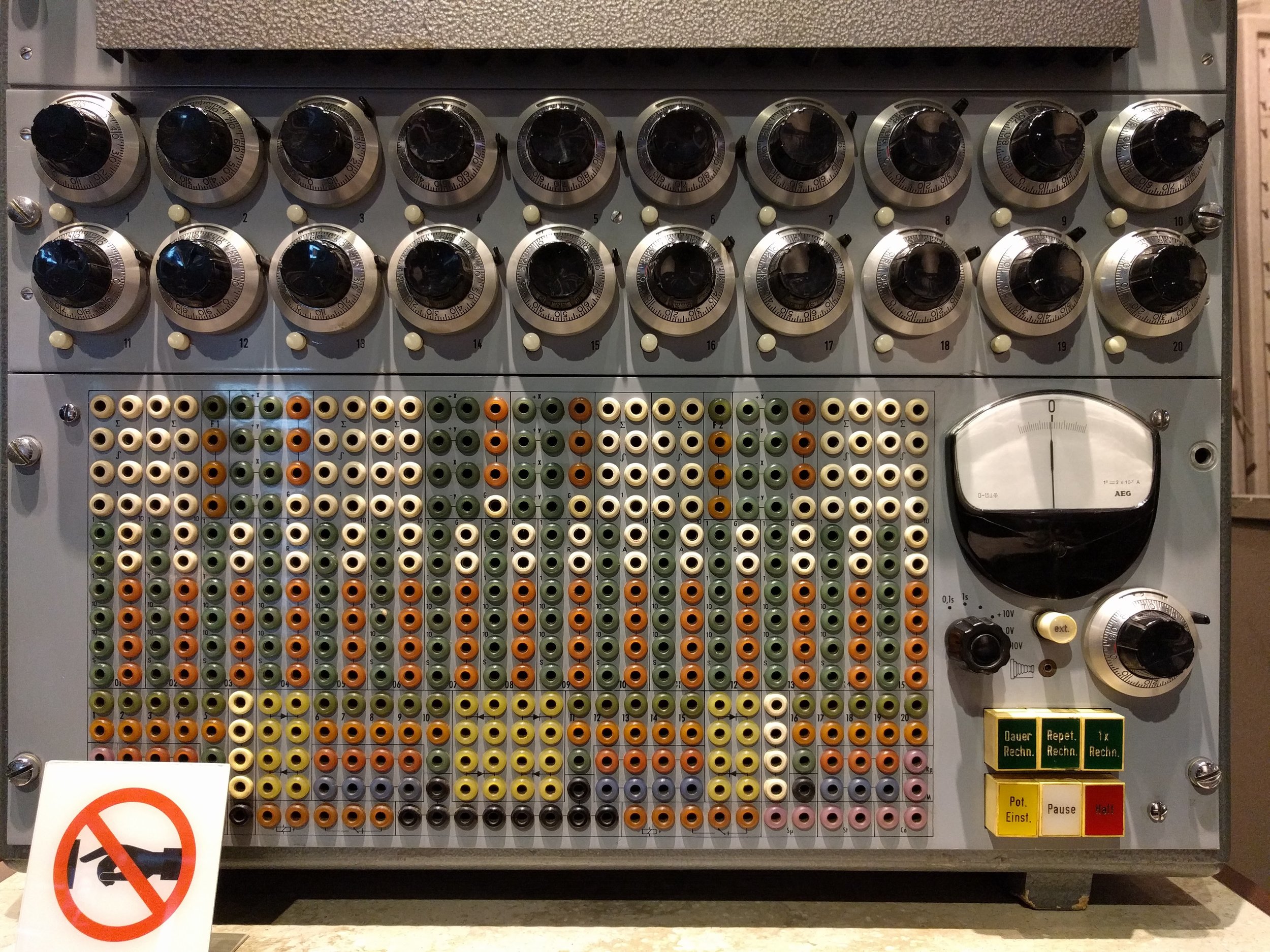
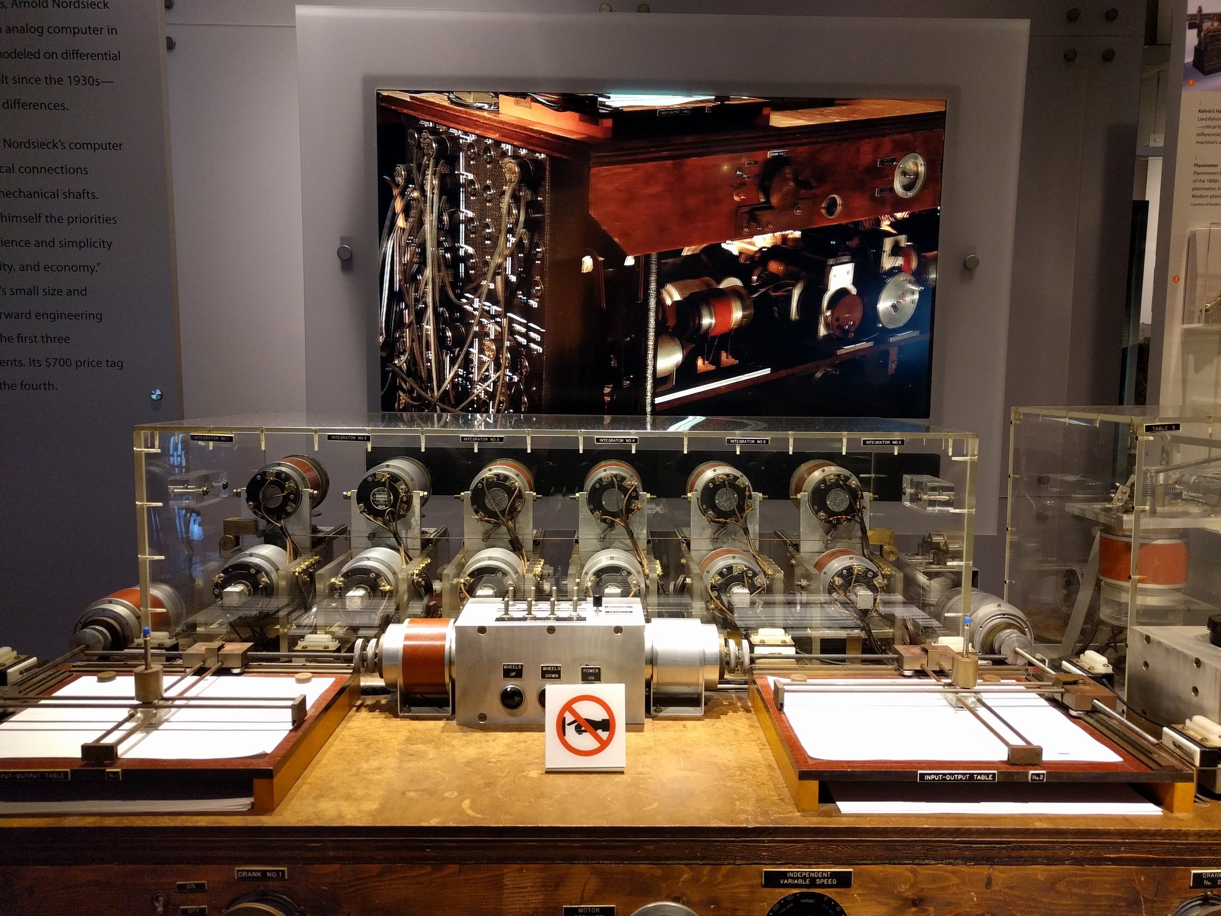
The Computer History Museum

View fullsize

Mountain View, California, looking northeast over US 101 and San Francisco Bay. The Computer History Museum sits between the Googleplex and NASA Ames. Hangar 1, the giant airship hangar, is visible on the right of the image. Imagery and map data © Google, Landsat/Copernicus.

A few days ago I was lucky enough to have a client meeting in Santa Clara, California. I had not been to Silicon Valley before, and it was more than a little exciting to drive down US Route 101 past the offices of Google, Oracle and Amazon and basically every other tech company, marvelling at Intel’s factory and the hangars at NASA Ames, and seeing signs to places like Stanford, Mountain View, and Menlo Park.

I had a spare day before I flew home, and decided to visit Stanford’s legendary geophysics department, where there was a lecture that day. With an hour or so to kill, I thought I’d take in the Computer History Museum on the way… I never made it to Stanford.

The museum

The Computer History Museum was founded in 1996, building on an ambition of über-geek Gordon Bell. It sits in the heart of Mountain View, surrounded by the Googleplex, NASA Ames, and Microsoft. It’s a modern, airy building with the museum and a small café downstairs, and meeting facilities on the upper floor. It turns out to be an easy place to burn four hours.

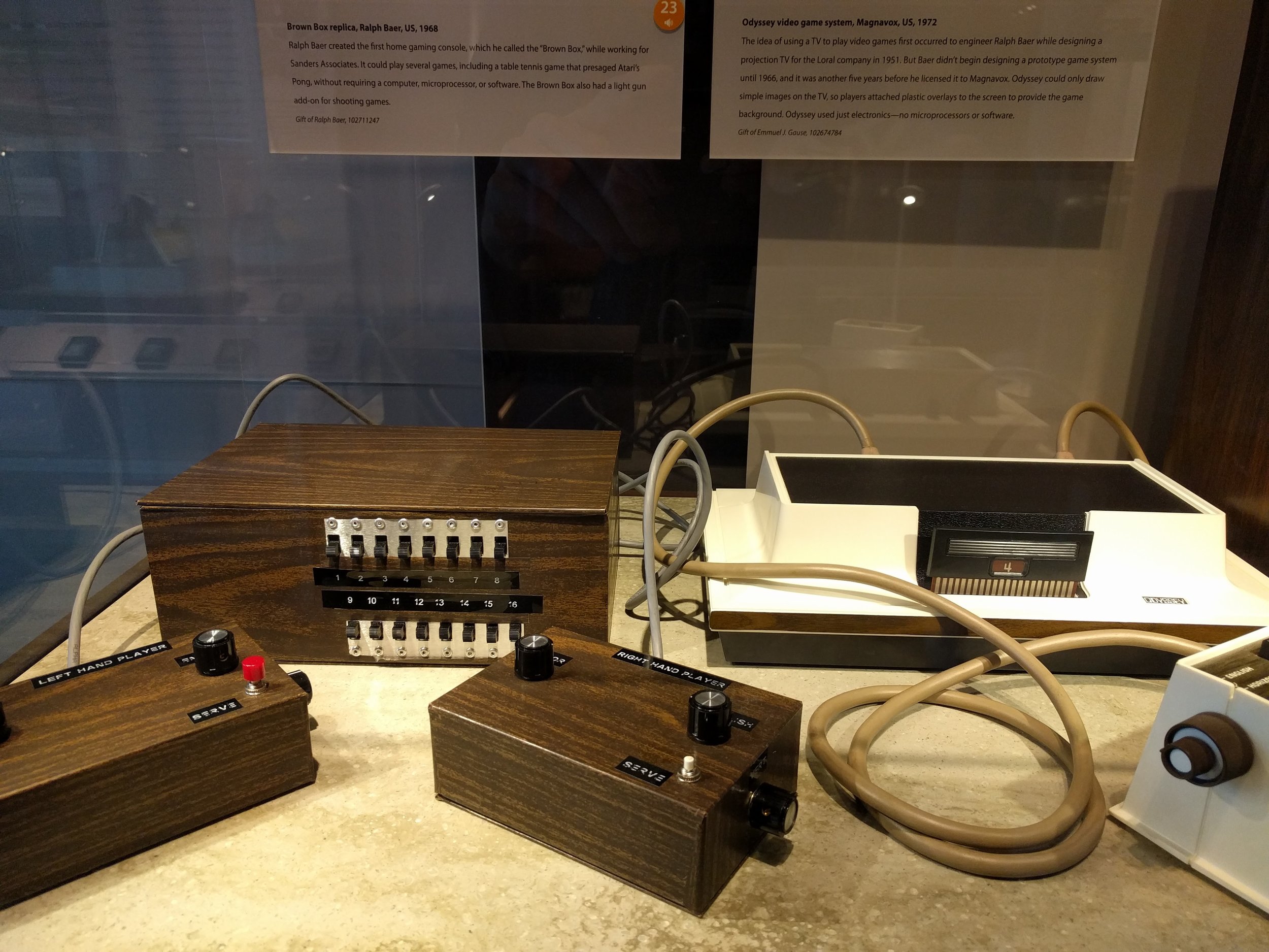
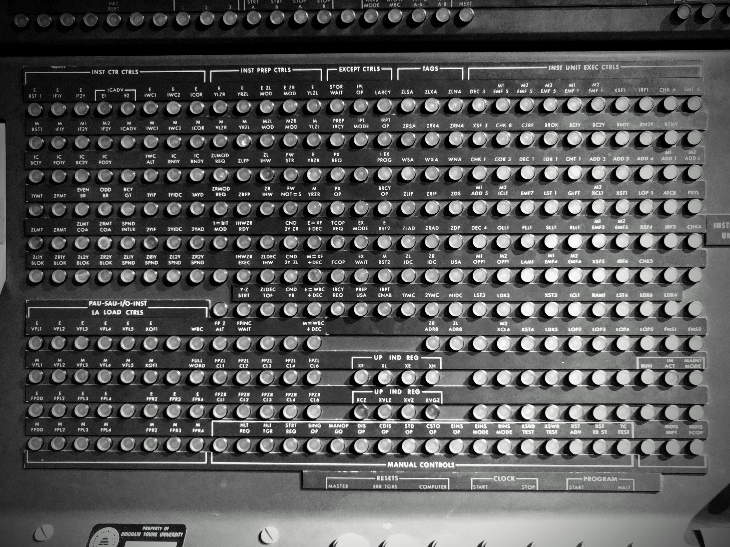
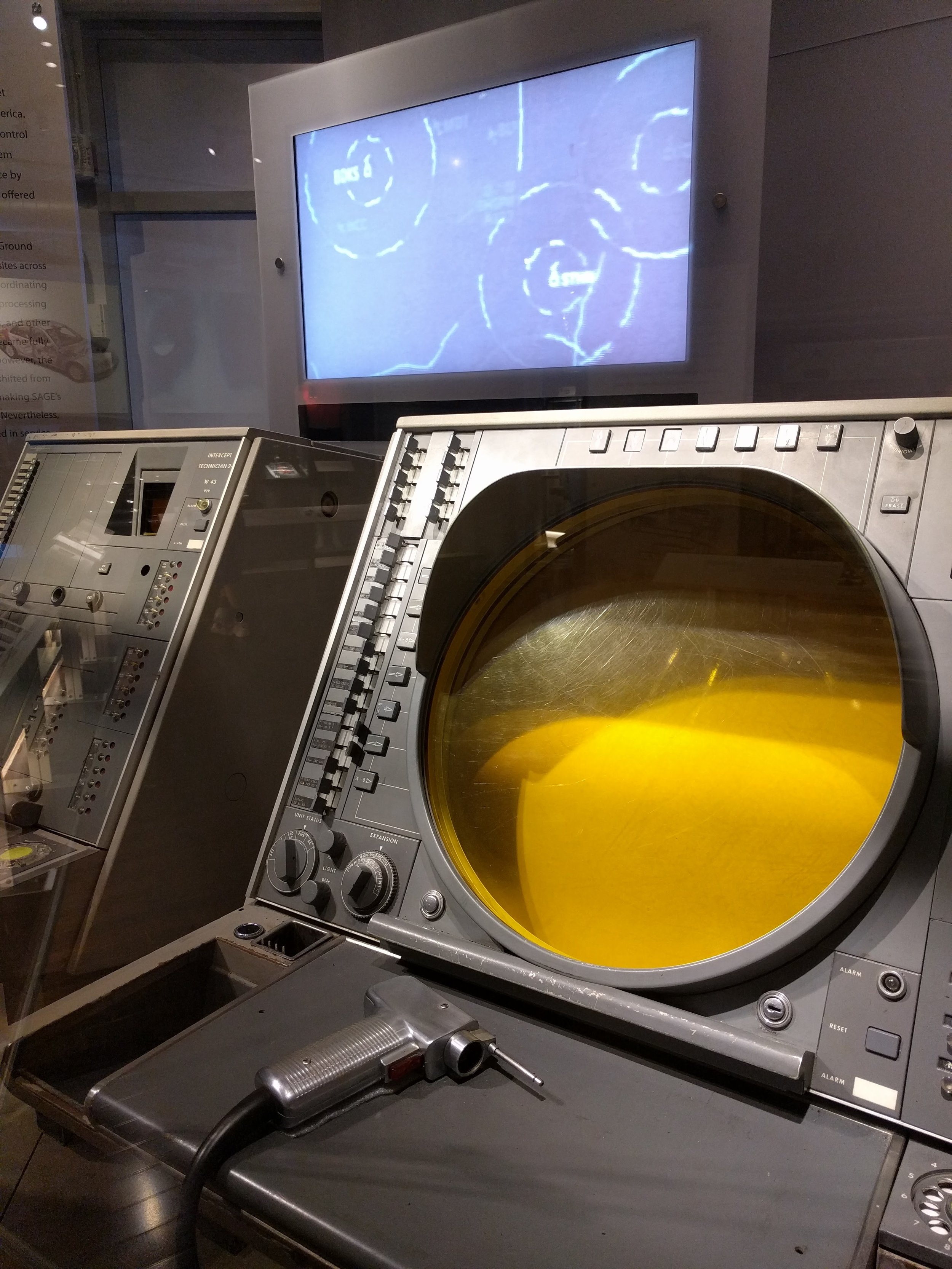
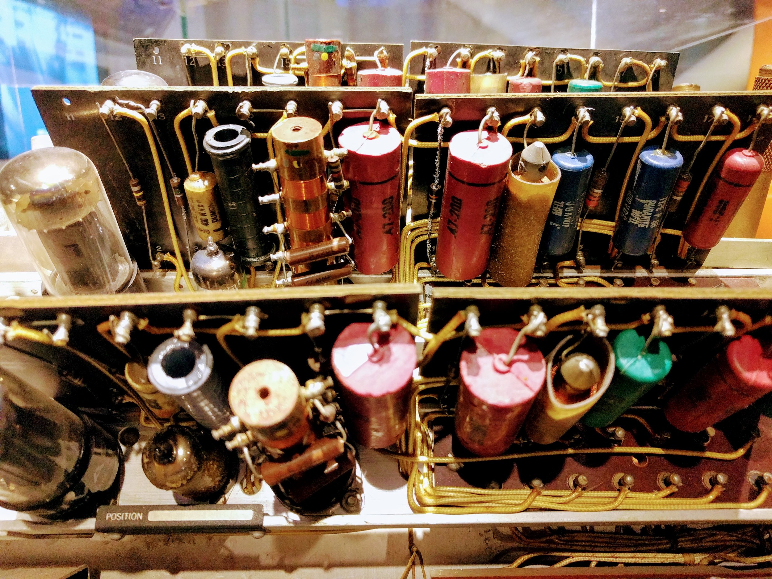
I saw a lot of computers that day. You can see them too because much of the collection is in the online catalog. A few things that stood out for me were:

• The analog computers of the pre-digital era, especially the beautiful Nordsieck Differential Analyzer.
• The actual, fully working, room-sized IBM 1401. Picture below.
• A wall of home computers from the early 1980s, including a BBC Micro and a ZX Spectrum, both important machines to me. The display even evoked the smell of those machines... and the frustration of reading programs from audio tapes.
• An Enigma machine, an Apple I, and Google’s actual server (just one rack!) from 1999, complete with its sagging motherboards.

View fullsize

No seismic

I had been hoping to read more about the early days of Texas Instruments, because it was spun out of a seismic company, Geophysical Service or GSI, and at least some of their early integrated circuit research was driven by the needs of seismic imaging. But I was surprised not to find a single mention of seismic processing in the place. We should help them fix this!

A replica of a 1968 game console. Nice finish!

1981 all over again.

You can't beat the aesthetic of early computers.

IBM's monolithic SAGE radar system. 

Gubbins.

Programming then was not like programming today.

An electronic analog computer, the Nordsieck Differential Analyzer (1950).

SEG machine learning contest: there's still time

Have you been looking for an excuse to find out what machine learning is all about? Or maybe learn a bit of Python programming language? If so, you need to check out Brendon Hall's tutorial in the October issue of The Leading Edge. Entitled, "Facies classification using machine learning", it's a walk-through of a basic statistical learning workflow, applied to a small dataset from the Hugoton gas field in Kansas, USA.

But it was also the launch of a strictly fun contest to see who can get the best prediction from the available data. The rules are spelled out in ther contest's README, but in a nutshell, you can use any reproducible workflow you like in Python, R, Julia or Lua, and you must disclose the complete workflow. The idea is that contestants can learn from each other.

View fullsize

Left: crossplots and histograms of wireline log data, coloured by facies — the idea is to highlight possible data issues, such as highly correlated features. Right: true facies (left) and predicted facies (right) in a validation plot. See the rest of the paper for details.

What's it all about?

The task at hand is to predict sedimentological facies from well logs. Such log-derived facies are sometimes called e-facies. This is a familiar task to many development geoscientists, and there are many, many ways to go about it. In the article, Brendon trains a support vector machine to discriminate between facies. It does a fair job, but the accuracy of the result is less than 50%. The challenge of the contest is to do better.

Indeed, people have already done better; here are the current standings:

	Team	F1	Algorithm	Language	Solution
1	gccrowther	0.580	Random forest	Python	Notebook
2	LA_Team	0.568	DNN	Python	Notebook
3	gganssle	0.561	DNN	Lua	Notebook
4	MandMs	0.552	SVM	Python	Notebook
5	thanish	0.551	Random forest	R	Notebook
6	geoLEARN	0.530	Random forest	Python	Notebook
7	CannedGeo	0.512	SVM	Python	Notebook
8	BrendonHall	0.412	SVM	Python	Initial score in article

As you can see, DNNs (deep neural networks) are, in keeping with the amazing recent advances in the problem-solving capability of this technology, doing very well on this task. Of the 'shallow' methods, random forests are quite prominent, and indeed are a great first-stop for classification problems as they tend to do quite well with little tuning.

How do I enter?

There is still over 6 weeks to enter: you have until 31 January. There is a little overhead — you need to learn a bit about git and GitHub, there's some programming, and of course machine learning is a massive field to get up to speed on — but don't be discouraged. The very first entry was from Bryan Page, a self-described non-programmer who dusted off some basic skills to improve on Brendon's notebook. But you can run the notebook right here in mybinder.org (if it's up today — it's been a bit flaky lately) and a play around with a few parameters yourself.

The contest aspect is definitely low-key. There's no money on the line — just a goody bag of fun prizes and a shedload of kudos that will surely get the winners into some awesome geophysics parties. My hope is that it will encourage you (yes, you) to have fun playing with data and code, trying to do that magical thing: predict geology from geophysical data.

---

Reference

Hall, B (2016). Facies classification using machine learning. The Leading Edge 35 (10), 906–909. doi: 10.1190/tle35100906.1. (This paper is open access: you don't have to be an SEG member to read it.)

Where is the ground?

This is the upper portion of a land seismic profile in Alaska. Can you pick a horizon where the ground surface is? Have a go at pickthis.io.

Pick the Ground surface at the top of the seismic section at pickthis.io.

Picking the ground surface on land-based seismic data is not straightforward. Picking the seafloor reflection on marine data, on the other hand, is usually a piece of cake, a warm-up pick. You can often auto-track the whole thing with a few seeds.

Seafloor reflection on Penobscot 3D survey, offshore Nova Scotia. from Matt's tutorial in the April 2016 The Leading Edge, The function of interpolation.

Why aren't interpreters more nervous that we don't know exactly where the surface of the earth is? I'm sure I'm not the only one that would like to have this information while interpreting. Wouldn't it be great if land seismic were more like marine?

Treacherously Jagged TopographY or Near-Surface processing ArtifactS?

If you're new to land-based seismic data, you might notice that there isn't a nice pickable event across the top of the section like we find in marine seismic data. Shot noise at the surface has been muted (deleted) in processing, and the low fold produces an unclean, jagged look at the top of the section. Additionally, the top of the section, time-zero — the seismic reference datum — usually floats somewhere above the land surface — and we can't know where that is unless it can be found in the file header, or looked up in the processing report.

The seismic reference datum, at a two-way time of zero seconds on seismic data, is typically set at mean sea level for offshore data. For land data, it is usually chosen to 'float' above the land surface.

Reframing the question

This challenge is a bit of a trick question. It begs the viewer to recognize that the seemingly simple task of mapping the ground level on a land seismic section is actually a rudimentary velocity modeling or depth conversion exercise in itself. Wouldn't it be nice to have the ground surface expressed as pickable seismic event? Shouldn't we have it always in our images? Baked into our data, so to speak, such that we've always got an unambiguous pick? In the next post, I'll illustrate what I mean and show what's involved in putting it in. 

In the meantime, I challenge you to pick where you think the (currently absent) ground surface is on this profile, so in the next post we can see how well you did.

x lines of Python: AVO plot

Amplitude vs offset (or, more properly, angle) analysis is a core component of quantitative interpretation. The AVO method is based on the fact that the reflectivity of a geological interface does not depend only on the acoustic rock properties (velocity and density) on both sides of the interface, but also on the angle of the incident ray. Happily, this angular reflectivity encodes elastic rock property information. Long story short: AVO is awesome.

As you may know, I'm a big fan of forward modeling — predicting the seismic response of an earth model. So let's model the response the interface between a very simple model of only two rock layers. And we'll do it in only a few lines of Python. The workflow is straightforward:

1. Define the properties of a model shale; this will be the upper layer.
2. Define a model sandstone with brine in its pores; this will be the lower layer.
3. Define a gas-saturated sand for comparison with the wet sand. 
4. Define a range of angles to calculate the response at.
5. Calculate the brine sand's response at the interface, given the rock properties and the angle range.
6. For comparison, calculate the gas sand's response with the same parameters.
7. Plot the brine case.
8. Plot the gas case.
9. Add a legend to the plot.

That's it — nine lines! Here's the result:

Once we have rock properties, the key bit is in the middle:

    θ = range(0, 31)
    shuey = bruges.reflection.shuey2(vp0, vs0, ρ0, vp1, vs1, ρ1, θ)

shuey2 is one of the many functions in bruges — here it provides the two-term Shuey approximation, but it contains lots of other useful equations. Virtually everything else in our AVO plotting routine is just accounting and plotting.

---

As in all these posts, you can follow along with the code in the Jupyter Notebook. You can view this on GitHub, or run it yourself in the increasingly flaky MyBinder (which is down at the time of writing... I'm working on an alternative).

What would you like to see in x lines of Python? Requests welcome!

What's that funny noise?

Seismic reflections are strange noises. Around 50 Hz, narrow band, very quiet, and difficult to interpret. It is possible to convert seismic traces (active or passive) into audible sound with a shift in pitch and a time stretch.

Made by the legendary Emory Cook, who recorded everything from steel bands to racing cars to ionospheric noises to this treatment of Hugo Benioff's earthquake recordings. Epic.

Curiously the audification thing has never really caught on in exploration geophysics — a bit surprising, given the fascination with spectral decomposition over the last 15 years or so. And especially so when you consider that our hearing has a dynamic range of about 100 dB, which is comparable to, indeed slightly greater than, our vision (about 90 dB).

Paolo Dell'Aversana of ENI wants to change that. Rather than listening to 'raw' seismic, he's sending it to a MIDI interface and listening to it as a piano roll. Just try to imagine playing seismic on a piano for a second, then listen to his weird and wonderful results — at 9:45 in this EAGE video:

In this EAGE E-Lecture Paolo Dell'Aversana discusses how digital music technology can support geophysical data analysis and interpretation. If you've read any of Dell'Aversana's articles, you'll know he has one of the most creative minds in exploration geophysics. Skip to 9:45 for the crazy seismic piano roll.

On the subject of weird sounds, one of my favourite Wikipedia pages is List of unexplained sounds. I especially love the eerie recordings of mysterious underwater noises, like this one called Upsweep:

No-one knows what makes that noise! My money's on a volcanic vent, but that doesn't explain the seasonality. Maybe we should do a hackathon on these unexaplained sounds some time. If you know of any others — I'd love tohear about them.

---

If you enjoy strange infrasound as much as I do, I recommend following these two scientists on Twitter:

• Milton Garces, aka Infrasound Hunter and director of the Infrasound LAb at the University of Hawaii.

• Stephen Gibbons, NORSAR seismologist who monitors nuclear testing with seismology.

---

If you really like strange noises, don't forget to check out the Undersampled Radio podcast!

Hooke's oolite

The new book

Hooke's engraving

Hooke's microscope

52 Things You Should Know About Rock Physics came out last week. For the first, and possibly the last, time a Fellow of the Royal Society — the most exclusive science club in the UK — drew the picture on the cover. The 353-year-old drawing was made by none other than Robert Hooke. 

The title page from Micrographia, and part of the dedication to Charles II. You can browse the entire book at archive.org.

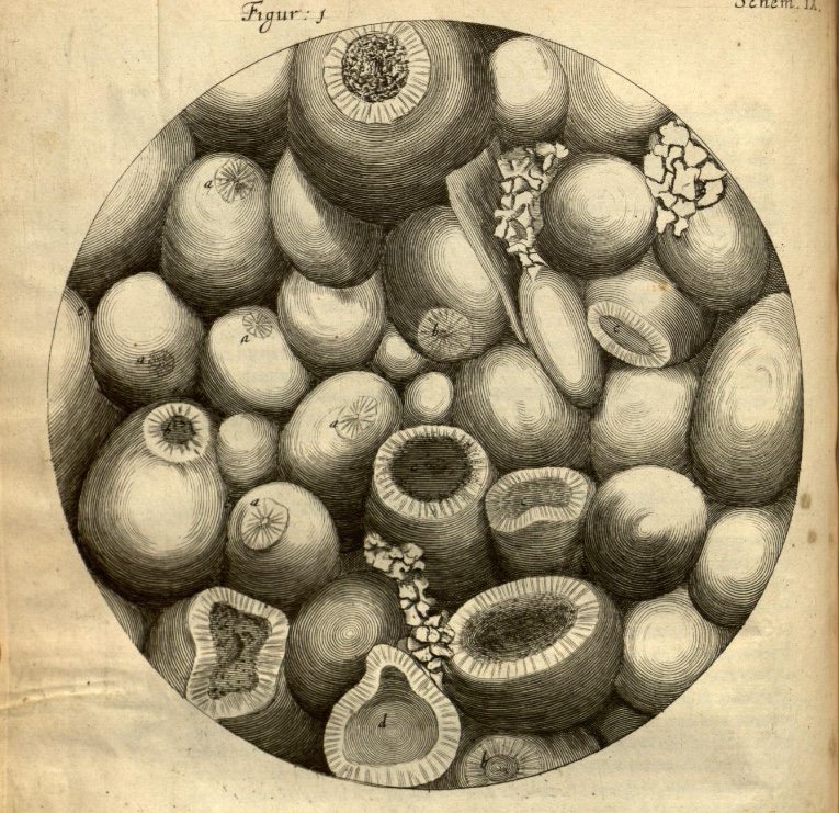
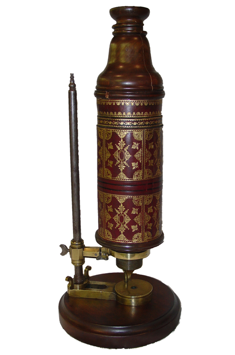
The drawing, or rather the engraving that was made from it, appears on page 92 of Micrographia, Hooke's groundbreaking 1665 work on microscopy. In between discovering and publishing his eponymous law of elasticity (which Evan wrote about in connection with Lamé's \(\lambda\)), he drew and wrote about his observations of a huge range of natural specimens under the microscope. It was the first time anyone had recorded such things, and it was years before its accuracy and detail were surpassed. The book established the science of microscopy, and also coined the word cell, in its biological context.

Sadly, the original drawing, along with every other drawing but one from the volume, was lost in the Great Fire of London, 350 years ago almost to the day. 

Ketton stone

The drawing on the cover of the new book is of the fractured surface of Ketton stone, a Middle Jurassic oolite from central England. Hooke's own description of the rock, which he mistakenly called Kettering Stone, is rather wonderful:

I wonder if anyone else has ever described oolite as looking like the ovary of a herring?

These thoughtful descriptions, revealing a profundly learned scientist, hint at why Hooke has been called 'England's Leonardo'. It seems likely that he came by the stone via his interest in architecture, and especially through his friendsip with Christopher Wren. By 1663, when it's likely Hooke made his observations, Wren had used the stone in the façades of several Cambridge colleges, including the chapels of Pembroke and Emmanuel, and the Wren Library at Trinity (shown here). Masons call porous, isotropic rock like Ketton stone 'freestone', because they can carve it freely to make ornate designs. Rock physics in action!

You can read more about Hooke's oolite, and the geological significance of his observations, in an excellent short paper by material scientist Derek Hull (1997). It includes these images of Ketton stone, for comparison with Hooke's drawing:

Reflected light photomicrograph (left) and backscatter scanning electron microscope image (right) of Ketton Stone. Adapted from figures 2 and 3 of Hull (1997). Images are © Royal Society and used in accordance with their terms.

I love that this book, which is mostly about the elastic behaviour of rocks, bears an illustration by the man that first described elasticity. Better still, the illustration is of a fractured rock — making it the perfect preface. 

---

Now at Amazon.com — Amazon.co.uk — Amazon.fr — Amazon.de — Amazon.it — Amazon.es
Soon at Amazon.ca — Amazon.com.mx — Amazon.com.br — Amazon.co.jp — Amazon.com.au — Amazon.in

---

References

Hall, M & E Bianco (eds.) (2016). 52 Things You Should Know About Rock Physics. Nova Scotia: Agile Libre, 134 pp.

Hooke, R (1665). Micrographia: or some Physiological Descriptions of Minute Bodies made by Magnifying Glasses, pp. 93–100. The Royal Society, London, 1665.

Hull, D (1997). Robert Hooke: A fractographic study of Kettering-stone. Notes and Records of the Royal Society of London 51, p 45-55. DOI: 10.1098/rsnr.1997.0005.

52 Things... Rock Physics

There's a new book in the 52 Things family! 

52 Things You Should Know About Rock Physics is out today, and available for purchase at Amazon.com. It will appear in their European stores in the next day or two, and in Canada... well, soon. If you can't wait for that, you can buy the book immediately direct from the printer by following this link.

The book mines the same vein as the previous volumes. In some ways, it's a volume 2 of the original 52 Things... Geophysics book, just a little bit more quantitative. It features a few of the same authors — Sven Treitel, Brian Russell, Rachel Newrick, Per Avseth, and Rob Simm — but most of the 46 authors are new to the project. Here are some of the first-timers' essays:

• Ludmilla Adam, Why echoes fade.
• Arthur Cheng, How to catch a shear wave.
• Peter Duncan, Mapping fractures.
• Paul Johnson, The astonishing case of non-linear elasticity.
• Chris Liner, Negative Q.
• Chris Skelt, Five questions to ask the petrophysicist.

It's our best collection of essays yet. We're very proud of the authors and the collection they've created. It stretches from childhood stories to linear algebra, and from the microscope to seismic data. There's no technical book like it. 

Supporting Geoscientists Without Borders

Purchasing the book will not only bring you profund insights into rock physics — there's more! Every sale sends $2 to Geoscientists Without Borders, the SEG charity that supports the humanitarian application of geoscience in places that need it. Read more about their important work.

It's been an extra big effort to get this book out. The project was completely derailed in 2015, as we — like everyone else — struggled with some existential questions. But we jumped back into it earlier this year, and Kara (the managing editor, and my wife) worked her magic. She loves working with the authors on proofs and so on, but she doesn't want to see any more equations for a while.

If you choose to buy the book, I hope you enjoy it. If you enjoy it, I hope you share it. If you want to share it with a lot of people, get in touch — we can help. Like the other books, the content is open access — so you are free to share and re-use it as you wish. 

Q is for Q

Quality factor, or \(Q\), is one of the more mysterious quantities of seismology. It's right up there with Lamé's \(\lambda\) and Thomsen's \(\gamma\). For one thing, it's wrapped up with the idea of attenuation, and sometimes the terms \(Q\) and 'attenuation' are bandied about seemingly interchangeably. For another thing, people talk about it like it's really important, but it often seems to be completely ignored.

A quick aside. There's another quality factor: the rock quality factor, popular among geomechnicists (geomechanics?). That \(Q\) describes the degree and roughness of jointing in rocks, and is probably related — coincidentally if not theoretically — to seismic \(Q\) in various nonlinear and probably profound ways. I'm not going to say any more about it, but if this interests you, read Nick Barton's book, Rock Quality, Seismic Velocity, Attenuation and Anistropy (2006; CRC Press) if you can afford it. 

So what is Q exactly?

We know intuitively that seismic waves lose energy as they travel through the earth. There are three loss mechanisms: scattering (elastic losses resulting from reflections and diffractions), geometrical spreading, and intrinsic attenuation. This last one, anelastic energy loss due to absorption — essentially the deviation from perfect elasticity — is what I'm trying to describe here.

I'm not going to get very far, by the way. For the full story, start at the seminal review paper entitled \(Q\) by Leon Knopoff (1964), which surely has the shortest title of any paper in geophysics. (Knopoff also liked short abstracts, as you see here.)

The dimensionless seismic quality factor \(Q\) is defined in terms of the energy \(E\) stored in one cycle, and the change in energy — the energy dissipated in various ways, such as fluid movement (AKA 'sloshing', according to Carl Reine's essay in 52 Things... Geophysics) and intergranular frictional heat ('jostling') — over that cycle:

$$ Q \stackrel{\mathrm{def}}{=} 2 \pi \frac{E}{\Delta E} $$

Remarkably, this same definition holds for any resonator, including pendulums and electronics. Physics is awesome!

Because the right-hand side of that relationship is sort of upside down — the loss is in the denominator — it's often easier to talk about \(Q^{-1}\) which is, more or less, the percentage loss of energy in a single wavelength. This inverse of \(Q\) is proportional to the attenuation coefficient. For more details on that relationship, check out Carl Reine's essay.

This connection with wavelengths means that we have to think about frequency. Because high frequencies have shorter cycles (by definition), they attenuate faster than low frequencies. You know this intuitively from hearing the beat, but not the melody, of distant music for example. This effect does not imply that \(Q\) depends on frequency... that's a whole other can of worms. (Confused yet?)

The frequency dependence of \(Q\)

It's thought that \(Q\) is roughly constant with respect to frequency below about 1 Hz, then increases with \(f^\alpha\), where \(\alpha\) is about 0.7, up to at least 25 Hz (I'm reading this in Mirko van der Baan's 2002 paper), and probably beyond. Most people, however, seem to throw their hands up and assume a constant \(Q\) even in the seismic bandwidth... mainly to make life easier when it comes to seismic processing. Attempting to measure, let alone compensate for, \(Q\) in seismic data is, I think it's fair to say, an unsolved problem in exploration geophysics.

Why is it worth solving? I think the main point is that, if we could model and measure it better, it could be a semi-independent measure of some rock properties we care about, especially velocity. Actually, I think it's even a stretch to call velocity a rock property — most people know that velocity depends on frequency, at least across the gulf of frequencies between seismic and acoustic logging tools, but did you know that velocity also depends on amplitude? Paul Johnson tells about this effect in his essay in the forthcoming 52 Things... Rock Physics book — stay tuned for more on that.

For a really wacky story about negative values of \(Q\) — which imply transmission coefficients greater than 1 (think about that) — check out Chris Liner's essay in the same book (or his 2014 paper in The Leading Edge). It's not going to help \(Q\) get any less mysterious, but it's a good story. Here's the punchline from a Jupyter Notebook I made a while back; it follows along with Chris's lovely paper:

Top: Velocity and the Backus average velocity in the E-38 well offshore Nova Scotia. Bottom: Layering-induced attenuation, or 1/Q, in the same well. Note the negative numbers! Reproduction of Liner's 2014 results in a Jupyter Notebook.

Hm, I had hoped to shed some light on \(Q\) in this post, but I seem to have come full circle. Maybe explaining \(Q\) is another unsolved problem.

References

Barton, N (2006). Rock Quality, Seismic Velocity, Attenuation and Anisotropy. Florida, USA: CRC Press. 756 pages. ISBN 9780415394413.

Johnson, P (in press). The astonishing case of non-linear elasticity.  In: Hall, M & E Bianco (eds), 52 Things You Should Know About Rock Physics. Nova Scotia: Agile Libre, 2016, 132 pp.

Knopoff, L (1964). Q. Reviews of Geophysics 2 (4), 625–660. DOI: 10.1029/RG002i004p00625.

Reine, C (2012). Don't ignore seismic attenuation. In: Hall, M & E Bianco (eds), 52 Things You Should Know About Geophysics. Nova Scotia: Agile Libre, 2012, 132 pp.

Liner, C (2014). Long-wave elastic attenuation produced by horizontal layering. The Leading Edge 33 (6), 634–638. DOI: 10.1190/tle33060634.1. Chris also blogged about this article.

Liner, C (in press). Negative Q. In: Hall, M & E Bianco (eds), 52 Things You Should Know About Rock Physics. Nova Scotia: Agile Libre, 2016, 132 pp.

van der Bann, M (2002). Constant Q and a fractal, stratified Earth. Pure and Applied Geophysics 159 (7–8), 1707–1718. DOI: 10.1007/s00024-002-8704-0.