2014 retrospective

At this time of year, we look back at the best of the blog — what were the most read, the most contentious, the most informative posts of the year? If you only stop by once every 12 months, this is the post for you!

Your favourites

Let's turn to the data first. Which posts got the most hits this year? Older posts have a time advantage of course, but here are the most popular new posts, starting with the SEG-Y double-bill:

• What is SEG-Y? and How to load SEG-Y, March
• It's the GGGG (giant geoscience gift guide), December
• Six books about seismic analysis, July

It's hard to say exactly how much attention a given post gets, because they sit on the front page of the site for a couple of weeks. Overall we got about 150 000 pageviews this year, and I think Well tie workflow — the most-read old post on the site this year — might have been read (okay, looked at) 5000 or so times.

I do love how some of our posts keep on giving: none of the top posts this year topped this year's readership of some golden oldies: Well tie workflow (written in April 2013), Six books about seismic interpretation (March 2013), k is for wavenumber (May 2012), Interpreting spectral gamma-ray logs (February 2013), or Polarity cartoons (April 2012).

What got people talking

When it all goes quiet on the comments, I worry that we're not provocative enough. But some posts provoke a good deal of chat, and always bring more clarity and depth to the issue. Don't miss the comments in Lusi's 8th birthday...

• Lusi's 8th birthday, 18 comments, mostly because of an epic argument.
• Data management fairy tales, 16 comments, and 10 ways to improve your data store, 12 comments.
• Are we alright? 13 comments, another contentious post.

Our favourites

We have our favourites too. Perhaps because a lot of work went into them (like Evan's posts about programming), or because they felt like important things to say (as in the 'two sides' post), or because they feel like part of a bigger idea.

Evan

• Well tie calculus
• Whither technical books?
• How much rock ... Mt St Helens?

Matt

• The new open geophysics tools
• Laying out a seismic survey
• Two sides to every story?

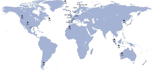
Where is everybody?

We don't collect detailed demographic data, but it's fun to see how people are reading, and roughly where they are. One surprise: the number of mobile readers did not rise this year — it's still about 15%. The top 10 cities were

1. Houston, USA
2. Calgary, Canada
3. London, UK
4. Perth, Australia
5. Ludwigshafen, Germany
6. Denver, USA
7. Aberdeen, UK
8. Moscow, Russia
9. Stavanger, Norway
10. Kuala Lumpur, Malaysia

Last thing

Thank You for reading! Seriously: we want to be a useful and interesting part of our community, so every glance at our posts, every comment, and every share, help us figure out how to be more useful and more interesting. We aim to get better still next year, with more tips and tricks, more code, more rants, and more conference reports — we look forward to sharing everything Agile with you in 2015.

If this week is Christmas for you, then enjoy the season. All the best for the new year!

Previous Retrospective posts... 2011 retrospective •  2012 retrospective • 2013 retrospective

Laying out a seismic survey

Cutlines for a dense 3D survey at Surmont field, Alberta, Canada. Image: Google Maps.

Cutlines for a dense 3D survey at Surmont field, Alberta, Canada. Image: Google Maps.There are a number of ways to lay out sources and receivers for a 3D seismic survey. In forested areas, a designer may choose a pattern that minimizes the number of trees that need to be felled. Where land access is easier, designers may opt for a pattern that is efficient for the recording crew to deploy and pick up receivers. However, no matter what survey pattern used, most geometries consist of receivers strung together along receiver lines and source points placed along source lines. The pairing of source points with live receiver stations comprises the collection of traces that go into making a seismic volume.

An orthogonal surface pattern, with receiver lines laid out perpendicular to the source lines, is the simplest surface geometry to think about. This pattern can be specified over an area of interest by merely choosing the spacing interval between lines well as the station intervals along the lines. For instance:

xmi = 575000        # Easting of bottom-left corner of grid (m)
ymi = 4710000       # Northing of bottom-left corner (m)
SL = 600            # Source line interval (m)
RL = 600            # Receiver line interval (m)
si = 100            # Source point interval (m)
ri = 100            # Receiver point interval (m)
x = 3000            # x extent of survey (m)
y = 1800            # y extent of survey (m)

We can calculate the number of receiver lines and source lines, as well as the number of receivers and sources for each.

# Calculate the number of receiver and source lines.
rlines = int(y/RL) + 1
slines = int(x/SL) + 1

# Calculate the number of points per line (add 2 to straddle the edges). 
rperline = int(x/ri) + 2 
sperline = int(y/si) + 2

# Offset the receiver points.
shiftx = -si/2.
shifty = -ri/2.

Computing coordinates

We create a list of x and y coordinates with a nested list comprehension — essentially a compact way to write 'for' loops in Python — that iterates over all the stations along the line, and all the lines in the survey.

# Find x and y coordinates of receivers and sources.
rcvrx = [xmi+rcvr*ri+shifty for line in range(rlines) for rcvr in range(rperline)]
rcvry = [ymi+line*RL+shiftx for line in range(rlines) for rcvr in range(rperline)]

srcx = [xmi+line*SL for line in range(slines) for src in range(sperline)]
srcy = [ymi+src*si for line in range(slines) for src in range(sperline)]

To make a map of the ideal surface locations, we simply pass this list of x and y coordinates to a scatter plot:

Plotting these lists is useful, but it is rather limited by itself. We're probably going to want to do more calculations with these points — midpoints, azimuth distributions, and so on — and put these data on a real map. What we need is to insert these coordinates into a more flexible data structure that can hold additional information.

Shapely, Pandas, and GeoPandas

Shapely is a library for creating and manipulating geometric objects like points, lines, and polygons. For example, Shapely can easily calculate the (x, y) coordinates halfway along a straight line between two points.

Pandas provides high-performance, easy-to-use data structures and data analysis tools, designed to make working with tabular data easy. The two primary data structures of Pandas are:

• Series — a one-dimensional labelled array capable of holding any data type (strings, integers, floating point numbers, lists, objects, etc.)
• DataFrame — a 2-dimensional labelled data structure where the columns can contain many different types of data. This is similar to the NumPy structured array but much easier to use.

GeoPandas combines the capabilities of Shapely and Pandas and greatly simplifies geospatial operations in Python, without the need for a spatial database. GeoDataFrames are a special case of DataFrames that are specifically for representing geospatial data via a geometry column. One awesome thing about GeoDataFrame objects is they have methods for saving data to shapefiles.

So let's make a set of (x,y) pairs for receivers and sources, then make Point objects using Shapely, and in turn add those to GeoDataFrame objects, which we can write out as shapefiles:

# Zip into x,y pairs.
rcvrxy = zip(rcvrx, rcvry)
srcxy = zip(srcx, srcy)

# Create lists of shapely Point objects.
rcvrs = [Point(x,y) for x,y in rcvrxy]
srcs = [Point(x,y) for x,y in srcxy]

# Add lists to GeoPandas GeoDataFrame objects.
receivers = GeoDataFrame({'geometry': rcvrs})
sources = GeoDataFrame({'geometry': srcs})

# Save the GeoDataFrames as shapefiles.
receivers.to_file('receivers.shp')
sources.to_file('sources.shp')

It's a cinch to fire up QGIS and load these files as layers on top of a satellite image or physical topography map. As a survey designer, we can now add, delete, and move source and receiver points based on topography and land issues, sending the data back to Python for further analysis.

All the code used in this post is in an IPython notebook. You can read it, and even execute it yourself. Put your own data in there and see how it comes out!

NEWSFLASH — If you think the geoscientists in your company would like to learn how to play with geological and geophysical models and data — exploring seismic acquisition, or novel well log displays — we can come and get you started! Best of all, we'll help you get up and running on your own data and your own ideas.

If you or your company needs a dose of creative geocomputing, check out our new geocomputing course brochure, and give us a shout if you have any questions. We're now booking for 2015.

The race for useful offsets

We've been working on a 3D acquisition lately. One of the factors influencing the layout pattern of sources and receivers in a seismic survey is the range of useful offsets over the depth interval of interest. If you've got more than target depth, you'll have more than one range of useful offsets. For shallow targets this range is limited to small offsets, due to direct waves and first breaks. For deeper targets, the range is limited at far offsets by energy losses due to geometric spreading, moveout stretch, and system noise.

In seismic surveying, one must choose a spacing interval between geophones along a receiver line. If phones are spaced close together, we can collect plenty of samples in a small area. If the spacing is far apart, the sample density goes down, but we can collect data over a bigger area. So there is a trade-off and we want to maximize both; high sample density covering the largest possible area.

What are useful offsets?

It isn't immediately intuitive why illuminating shallow targets can be troublesome, but with land seismic surveying in particular, first breaks and near surface refractions clobber shallow reflecting events. In the CMP domain, these are linear signals, used for determining statics, and are discarded by muting them out before migration. Reflections that arrive later than the direct wave and first refractions don't get muted out. But if these reflections arrive later than the air blast noise or ground roll noise — pervasive at near offsets — they get caught up in noise too. This region of the gather isn't muted like the top mute, otherwise you'd remove the data at near offsets. Instead, the gathers are attacked with algorithms to eliminate the noise. The extent of each hyperbola that passes through to migration is what we call the range of useful offsets.

The deepest reflections have plenty of useful offsets. However if we wanted to do adequate imaging somewhere between the first two reflections, for instance, then we need to make sure that we record redundant ray paths over this smaller range as well. We sometimes call this aperture; the shallow reflection is restricted in the number of offsets that it can be illuminated with, the deeper reflections can tolerate an aperture that is more open. In this image, I'm modelling the case of 60 geophones spanning 3000 metres, spaced evenly at 100 metres apart. This layout suggests merely 4 or 5 ray paths will hit the uppermost reflection, the shortest ray paths at small offsets. Also, there is usually no geophone directly on top of the source location to record a vertical ray path at zero offset. The deepest reflections however, should have plenty of fold, as long as NMO stretch, geometric spreading, and noise levels were good.

The problem with determining the range of useful offsets by way of a model is, not only does it require a velocity profile, which is easily attained from a sonic log, VSP, or velocity analysis, but it also requires an estimation of the the speed, intensity, and duration of the near surface events to be muted. Parameters that depend largely on the nature of the source and the local ground conditions, which vary from place to place, and from one season to the next.

In a future post, we'll apply this notion of useful offsets to build a pattern for shooting a 3D.

---

Click here for details on how I created this figure using the IPython Notebook. If you don't have it, IPython is easy to install. The easiest way is to install all of scientific Python, or use Canopy or Anaconda.

This post was inspired in part by Norm Cooper's 2004 article, A world of reality: Designing 3D seismic programs for signal, noise, and prestack time-migration. The Leading Edge23 (10), 1007-1014.DOI: 10.1190/1.1813357

Update on 2014-12-17 13:04 by Matt Hall
Don't miss the next installment — Laying out a seismic survey — with more IPython goodness!

The new open geophysics tools

The hackathon in Denver was more than 6 weeks ago. I kept thinking, "Oh, I must post a review of what went down" (beyond the quick wrap-up I did at the time), but while I'm a firm believer in procrastination six weeks seems unreasonable... Maybe it's taken this long to scrub down to the lasting lessons. Before those, I want to tell you who the teams were, what they did, and where you can find their (100% open source!) stuff. Enjoy!

Geophys Wiz

Andrew Pethick, Josh Poirier, Colton Kohnke, Katerina Gonzales, and Elijah Thomas — GitHub repo

This team had no trouble coming up with ideas — perhaps a reflection of their composition, which was more heterogeneous than the other teams. Josh is at NEOS, the consulting and software firm, and Andrew is a postdoc at Curtin in Perth, Australia, while the other 3 are students at Mines. The team eventually settled on building MT Black Box, a magnetotellurics modeling web application. 

Last thing: Don't miss Andrew Pethick's write-up of the event. 

Seemingly Concerned Neighbours

Elias Arias, Brent Putman, Thomas Rapstine, and Gabriel Martinez — Github repo

These four young geophysicists from the Colorado School of Mines impressed everyone with their work ethic. Their tight-knit team came in with a plan, and proceeded to scribble up the coolest-looking whiteboard of the weekend. After learning some Android development skills 'earlier this week', they pulled together a great little app for forward modeling magnetotelluric responses. 

Well tie guys

Michaël Montouchet, Graham Dawes, Mark Roberts

It was terrific to have pro coders Graham and Michaël with us — they flew from the UK to be with us, thanks to their employer and generous sponsor ffA GeoTeric. They hooked up with Mark, a Denver geophysicist and developer, and hacked on a well-tie web application, rightly identifying a gap in the open source market, so to speak (there is precious little out there for well-based workflows). They may have bitten off more than they could chew in just 2 days, so I hope we can get together with them again to finish it off. Who's up for a European hackathon? 

Five hour wonders

Rowan Cockett and Seogi Kang — GitHub repo for SimPEG

These two characters from UBC didn't get going till Sunday morning, but in just five hours they built a sweet web app for forward modeling the DC resistivity response of a buried disk. They weren't starting from scratch, because Rowan and others have spent months honing SimPEG, a rich open-source geophysical library, but minds were nonetheless blown.

Key takeaway: interactivity beyond sliders for the win.

Pick This!

Ben Bougher, Jacob Foshee, Evan Bianco, and an immiscible mixture of Chris Chalcraft and me — GitHub repo

Wouldn't you sometimes like to know how other people would interpret the section you're working on? This team, a reprise of the dream team from Houston in 2013, built a simple way to share images and invite others to interpret them. When someone has completed their interpretation, only then do they get to see the ensemble — everyone else's interpretations — in a heatmap. Not only did this team demo live software at pickthis.io, but the audience provided the first crowdsourced picks in real time. 

We'll be blogging more about Pick This soon. We're actively seeking ideas, images, interpreters, and financial support. Keep an eye out.

What I learned at this hackathon

• Potential fields are an actual thing! OK, kidding, but three out of five teams built potential field modeling tools. I wasn't expecting that, and I think the judges were impressed at the breadth. 
• 30 hours is easily enough time to build something pretty cool. Heck, 5 hours is enough if you're made of the right stuff. 
• Students can happily build prototypes alongside professional developers, and even teach them a thing or two. And vice versa. Are hackathons a leveller of playing fields?
• We need to remove the road blocks to more people enjoying this event. To help with this, next time there will be a 1-day bootcamp before the hackathon.
• After virtually doubling in size from 2013 to 2014, it's clear that the 2015 Hackathon in New Orleans is going to be awesome! Mark your calendar: 17 and 18 October 2015.

Thank you!

Thank you to the creative, energetic geophysicists that came. It was a privilege to meet and hack with you!

Thank you to the judges who gave up their Sunday teatime to watch the demos and give precious feedback to the teams: Steve Adcock, Jamie Allison, Maitri Erwin, Dennis Cooke, Chris Krohn, Shannon Bjarnason, David Holmes, and Tracy Stark. Amazing people, one and all.

A final Thank You to our sponsors — dGB Earth Sciences, ffA GeoTeric, and OpenGeoSolutions. You guys are totally awesome! Seriously.

It's the GGGG (giant geoscience gift guide)

I expect you've been wondering what to get me and Evan for Christmas. Wonder no more! Or, if you aren't that into Agile, I suppose other geoscientists might even like some of this stuff. If you're feeling more needy than generous, just leave this post up on a computer where people who love you will definitely see it, or print it out and mail it to everyone you know with prominent red arrows pointing to the things you like best. That's what I do.

Geology in the home

• If there is a finer object than this amazing table, I don't know what it is. This rifted table tries to challenge, but the winner is clear.
• I suppose this wonderful Little River is at least more sedimentological.
• You can have a stratigraphic rug or two...
• ...some petrological wallpaper...
• ...or even a volcanological pillow of the non-lava variety.
• Geophysicists love plates. Here are some beauties with waves.

Art!

• This vintage mineral poster is completely awesome. Here's another. There are cards too.
• How about some paleoart from Winnipeg artist Julius Csotonyi? If trilobitic surrealism is more your genre, then Glendon Mellow is your man.
• I don't know if you'd call it art, but Shapeways has all sorts of 3D-printed treasures, like a T Rex skull, or a model of Comet Churyumov–Gerasimenko. Or make your own models with this crazy 3D printing pen.
• I'm still waiting for someone to get me this glass seismograph by Andy Paiko, which might be the actual greatest thing ever... even better than that table.

Museums and trips and stuff

• Give to the Royal Tyrrell Museum in Drumheller, Alberta, one of the world's leading dinosaur research centres.
• I went to Iceland and my kids thought it was the best place ever. Go there! Get inside a volcano!
• Go and look for dinosaur tracks in Wyoming — riding a giant mammal of your choice! Well, a horse.

Image is CC-BY by Greg Westfall on Flickr

Geo-apparel

• An ugly tie for geologists you like, but not like like. If it's true love, Spoonflower has a lot of geological fabric you can make stuff out of. You will never touch the original seismic well tie, however.
• This is one of the better geological pun T-shirts, an oft-mined vein. There are lotsofothers.
• I think this onesie only comes in infant sizes. But no worries, babies need rocking threads too!  

Blimey... books!

Who over the age of 21 or maybe 30 doesn't love getting books for Christmas? I don't!... not love it. Er, anyway, here are some great reads!

• How about 156 things for the price of three? Yeah, that is a deal.
• They're not geological but my two favourite books of the year were highly geeky — What If? by Randall Munroe and Cool Tools by Kevin Kelly.
• Let's face it, you're going to get books for the kids in your life too (I hope). You can't do better than Jon Tennant's Excavate! Dinosaurs.
• You're gonna need some bookends for all these books.

Still stuck? Come on!

• Travel back in time to 2013, 2012, or 2011 for previous editions of this awesome gift guide. 
• Check out what the Natural History Museum or Smithsonian have on offer.
• Last year the EGU Geolog blog and the ever-reliable Evelyn Mervine had great ideas too.

---

All of the smaller images in this post are copyright of their respective owners, and I'm hoping they don't mind me using them to help sell their stuff.

Update on 2014-12-12 01:41 by Matt Hall
​In case you're still struggling, Evelyn Mervine has posted her annual list over on the AGU Blogosphere. If you find any more geo-inspired gift lists, or have ideas for others, please drop them in the comments.

Neglected near-surface workhorses

Yesterday afternoon, I attended a talk at Dalhousie by Peter Cary who has begun the CSEG distinguished lecture tour series. Peter's work is well known in the seismic processing world, and he's now spreading his insights to the broader geoscience community. This was only his fourth stop out of 26 on the tour, so there's plenty of time to catch it.

Three steps of seismic processing

In the head-spinning jargon of seismic processing, if you're lost, it's maybe not be your fault. Sometimes it might even seem like you're going in circles.

Ask the vendor or processing specialist first to keep it simple, and second to tell you in which of the three processing stages you are in. Seismic data processing has steps:

• Attenuate all types of noise.
• Remove the effects of the near surface.
• Migration, sometimes called imaging.

If time migration is the workshorse of seismic processing, and if is f–k filtering (or f–anything filtering) is the workhorse of noise attenuation, then surface consistent deconvolution is the workhorse of the near surface. These topics aren't as sexy or as new as FWI or compressed sensing, but Peter has been questioning the basics of surface-consistent scaling, and the approximations we make when processing land seismic data. 

The ambiguity of phase and travel-time corrections

To the processor, removing the effects of the near surface means making things flat in the CMP domain. It turns out you can do this with travel time corrections (static shifts), you can do this with phase corrections, or you can do it with both.

A simple synthetic example showing (a) a gather with surface-consistent statics and phase variations; (b) the same gather after surface-consistent residual statics correction, and (c) after simultaneous surface-consistent statics and phase correcition. Image © Cary & Nagarajappa and CSEG.

It's troubling that there is more than one way to achieve flatness. Peter's advice is to use shot stacks and receiver stacks to compare the efficacy of static corrections. They eliminate doubt about whether surface consistent scaling is working, and are a better QC tool than other data domains.

Deeper than shallow

It may sound trivial, but the hardest part about using seismic waves for imaging is that they have to travel down and back up through the near surface on their path to the target. It might seem counter-intuitive, but the geometric configurations that work well for the deep earth are not well suited to the shallow earth, and how we might correct for it. I can imagine that two surveys could be useful, one for the target and one for characterizing the shallow that gets in the way of the target, but seismic experiments are already expensive enough when there is only target to be concerned with.

Still, the near surface is something we can't avoid. Much like astronomers using ground-based telescopes shooting for the stars, seismic processors too have to get the noisy stuff that is sitting closest to the detectors out of the way.

Another 52 Things hits the shelves

The new book is out today: 52 Things You Should Know About Palaeontology. Having been up for pre-order in the US, it is now shipping. The book will appear in Amazons globally in the next 24 hours or so, perhaps a bit longer for Canada.

I'm very proud of this volume. It shows that 52 Things has legs, and the quality is as high as ever. Euan Clarkson knows a thing or two about fossils and about books, and here's what he thought of it: 

This is sheer delight for the reader, with a great range of short but fascinating articles; serious science but often funny. Altogether brilliant!

Each purchase benefits The Micropalaeontological Society's Educational Trust, a UK charity, for the furthering of postgraduate education in microfossils. You should probably go and buy it now before it runs out. Go on, I'll wait here...

1000 years of fossil obsession

So what's in the book? There's too much variety to describe. Dinosaurs, plants, foraminifera, arthropods — they're all in there. There's a geographical index, as before, and also a chronostratigraphic one. The geography shows some distinct clustering, that partly reflects the emphasis on the science of applied fossil-gazing: biostratigraphy. 

The book has 48 authors, a new record for these collections. It's an honour to work with each of them — their passion, commitment, and professionalism positively shines from the pages. Geologists and fossil nuts alike will recognize many of the names, though some will, I hope, be new to you. As a group, these scientists represent  1000 years of experience!

---

Amazingly, and completely by chance, it is one year to the day since we announced 52 Things You Should Know About Geology. Sales of that book benefit The AAPG Foundation, so today I am delighted to be sending a cheque for $1280 to them in Tulsa. Thank you to everyone who bought a copy, and of course to the authors of that book for making it happen.

Imaging with vectors

Even though it took way too long (I had been admiring it for quite some time), I recently became the first kid on the block to own a Lytro. The Lytro, if you haven't heard, is sort of like a camera, except that it definitely isn't. Apart from a viewfinder on one end, a piece of glass on the other, and a shutter release button on top, it doesn't really look or feel like a point-and-shoot or SLR either. It actually bares a closer resemblance to a pocket-sized telescope. So don't you dare call it a camera. Indeed, the thing that the Lytro is built to do is what makes it completely different than any camera, and this perhaps, is the best mark of its identity. It captures not only the intensity of the light rays hitting the sensor (or film), but the directionality of those light rays as well.

So what. Right? What does this mean? Why is this interesting? It means that with a light-field camera, the focal point and depth of field are parameters that can be controlled by the viewer. It is interesting because of freeing up of space and of the physical atoms of hardware by deliberately removing the motorized auto-focus mechanism, and placing instead into the capable and powerful hands of software. I find it particularly elegant that this technology was acheived as a result of harnessing light's true nature better than any other camera that came before it. A device designed to to record light as light is; a physical property defined by both a magnitude and a direction.

How do I interact with this picture? 

Normally this would be a weird question to ask, but with the Lytro the viewer can take part in the imaging process in three ways. Try it out on the samples above:

• Point to focus: collecting the light field from a scene is a technical thing. Creating images by deciding what to focus on, and what to not focus on is an artistic thing. It is an interpretive thing. It's a narrative that the viewer has with the data. The goal of the light field camera is not to impose a narrative, but instead get entirely out of the way.
• Extended focus: for artistic reasons, the viewer might want to have some parts of the image in focus, other parts out of focus. It's how our eyes work; our peripheral vision. But in cases where you want to see the full depth of field, where everything is in focus, the software has an algorithm for that (to try it out you can press 'E' on your keyboard).
• Stereo viewing: speaks to the multidimensional nature of the vector field data. In the real world, when we move our head, the foreground moves faster than the background. So too with light-field images, you can simulate parallax, by moving your cursor and better understand the spatial relationship between objects in the scene.

These capabilities aren't just components of the device, they are technological paradigms embodied by the device. That, to me, is what is so incredibly beautiful about this technology. It's the best example of what technology should be: a material thing that improves the work of the mind.

A call to the seismic industry

The seismic wavefield is what we should be giving to the interpreter. This probably means engineering a seismic system where less work is done by the processor, and more control is given to the interpreter through software that does the heavy lifting. Interpreters need to have direct feedback with the medium they are interpreting. How does seismic have to change to allow that narrative?

R is for Resolution

Resolution is becoming a catch-all term for various aspects of the quality of a digital signal, whether it's a photograph, a sound recording, or a seismic volume.

I got thinking about this on seeing an ad in AAPG Explorer magazine, announcing an 'ultra-high-resolution' 3D in the Gulf of Mexico (right), aimed at site-survey and geohazard detection. There's a nice image of the 3D, but the only evidence offered for the 'ultra-high-res' claim is the sample interval in space and time (3 m × 6 m bins and 0.25 ms sampling). This is analogous to the obsession with megapixels in digital photography, but it is only one of several ways to look at resolution. The effect of increasing the sample interval of some digital images is shown in the second column here, compared to 200 × 200 pixels originals (click to zoom):

Another aspect of resolution is spatial bandwidth, which gets at resolving power, perhaps analogous to focus for a photographer. If the range of frequencies is too narrow, then broadband features like edges cannot be represented. We can simulate poor frequency content by bandpassing the data, for example smoothing it with a Gaussian filter (column 3).

Yet another way to think about resolution is precision (column 4). Indeed, when audiophiles talk about resolution, they are talking about bit depth. We usually record seismic with 32 bits per sample, which allows us to discriminate between a large number of values — but we often view seismic with only 6 or 8 bits of precision. In the examples here, we're looking at 2 bits. Fewer bits means we can't tell the difference between some values, especially as it usually results in clipping.

If it comes down to our ability to tell events (or objects, or values) apart, then another factor enters the fray: signal-to-noise ratio. Too much noise (column 5) impairs our ability to resolve detail and discriminate between things, and to measure the true value of, say, amplitude. So while we don't normally talk about the noise level as a resolution issue, it is one. And it may have the most variety: in seismic acquisition we suffer from thermal noise, line noise, wind and helicopters, coherent noise, and so on.

I can only think of one more impairment to the signals we collect, and it may be the most troubling: the total duration or extent of the observation (column 6). How much information can you afford to gather? Uncertainty resulting from a small window is the basis of the game Name That Tune. If the scale of observation is not appropriate to the scale we're interested in, we risk a kind of interpretation 'gap' — related to a concept we've touched on before — and it's why geologists' brains need to be helicoptery. A small 3D is harder to interpret than a large one. 

The final consideration is not a signal effect at all. It has to do with the nature of the target itself. Notice how tolerant the brick wall image is to the various impairments (especially if you know what it is), and how intolerant the photomicrograph is. In the astronomical image, the galaxy is tolerant; the stars are not. Notice too that trying to 'resolve' the galaxy (into a point, say) would be a mistake: it is inherently low-resolution. Indeed, its fuzziness is one of its salient features.

Have I missed anything? Are there other ways in which the recorded signal can suffer and targets can be confused or otherwise unresolved? How does illumination fit in here, or spectral bandwidth? What do you mean when you talk about resolution?

---

This post is an exceprt from my talk at SEG, which you can read about in this blog post. You can even listen to it if you're really bored. The images were generated by one of my IPython Notebooks that I point to in the talk, specifically images.ipynb. 

Astute readers with potent memories will have noticed that we have skipped Q in our A to Z. I just cannot seem to finish my post about Q, but I will!

The Safe Band ad is copyright of NCS SubSea. This low-res snippet qualifies as fair use for comment.

All the time freaks

Thursday was our last day at the SEG Annual Meeting. Evan and I took in the Recent developments in time-frequency analysis workshop, organized by Mirko van der Baan, Sergey Fomel, and Jean-Baptiste Tary (Vienna). The workshop came out of an excellent paper I reviewed this summer, which was published online a couple of weeks ago:

Tary, JB, RH Herrera, J Han, and M van der Baan (2014), Spectral estimation—What is new? What is next?, Rev. Geophys. 52. doi:10.1002/2014RG000461.

The paper compares the results of several time–frequency transforms on a suite of 'benchmark' signals. The idea of the workshop was to invite further investigation or other transforms. The organizers did a nice job of inviting contributors with diverse interests and backgrounds. The following people gave talks, several of them sharing their code (*):

• John Castagna (Lumina) with a review of the applications of spectral decomposition for seismic analysis.
• Steven Lin (NCU, Taiwan) on empirical methods and the Hilbert–Huang transform.
• Hau-Tieng Wu (Toronto) on the application of transforms to monitoring respiratory patterns in animals.*
• Marcílio Matos (SISMO) gave an entertaining, talk about various aspects of the problem.
• Haizhou Yang (Standford) on synchrosqueezing transforms applied to problems in anatomy.*
• Sergey Fomel (UT Austin) on Prony's method... and how things don't always work out.*
• Me, talking about the fidelity of time–frequency transforms, and some 'unsolved problems' (for me).*
• Mirko van der Baan (Alberta) on the results from the Tary et al. paper.

Some interesting discussion came up in the two or three unstructured parts of the session, organized as mini-panel discussions with groups of authors. Indeed, it felt like the session could have lasted longer, because I don't think we got very close to resolving anything. Some of the points I took away from the discussion:

• My observation: there is no existing survey of the performance of spectral decomposition (or AVO) — these would be great risking tools.
• Castagna's assertion: there is no model that predicts the low-frequency 'shadow' effect (confusingly it's a bright thing, not a shadow).
• There is no agreement on whether the so-called 'Gabor limit' of time–frequency localization is a lower-bound on spectral decomposition. I will write more about this in the coming weeks.
• Should we even be attempting to use reassignment, or other 'sharpening' tools, on broadband signals? To put it another way: does instantaneous frequency mean anything in seismic signals?
• What statistical measures might help us understand the amount of reassignment, or the precision of time–frequency decompositions in general?

The fidelity of time–frequency transforms

My own talk was one of the hardest I've ever done, mainly because I don't think about these problems very often. I'm not much of a mathematician, so when I do think about them, I tend to have more questions than insights, so I made my talk into a series of questions for the audience. I'm not sure I got much closer to any answers, but I have a better idea of my questions now... which is a kind of progress I suppose.

Here's my talk (latest slides — GitHub repo). Comments and feedback are, as always, welcome.