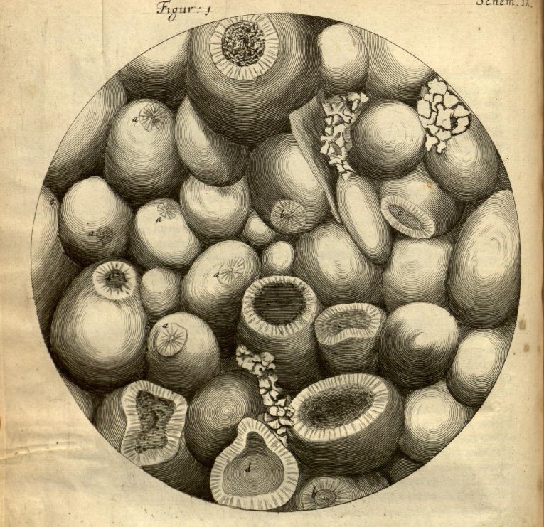
Hooke's oolite

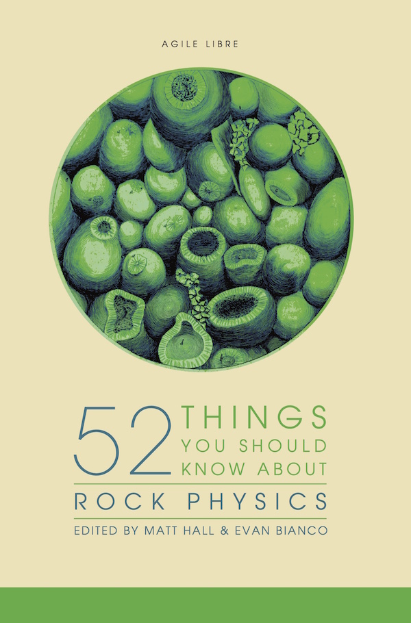
52 Things You Should Know About Rock Physics came out last week. For the first, and possibly the last, time a Fellow of the Royal Society — the most exclusive science club in the UK — drew the picture on the cover. The 353-year-old drawing was made by none other than Robert Hooke

The title page from Micrographia, and part of the dedication to Charles II. You can browse the entire book at archive.org.

The title page from Micrographia, and part of the dedication to Charles II. You can browse the entire book at archive.org.

The drawing, or rather the engraving that was made from it, appears on page 92 of Micrographia, Hooke's groundbreaking 1665 work on microscopy. In between discovering and publishing his eponymous law of elasticity (which Evan wrote about in connection with Lamé's \(\lambda\)), he drew and wrote about his observations of a huge range of natural specimens under the microscope. It was the first time anyone had recorded such things, and it was years before its accuracy and detail were surpassed. The book established the science of microscopy, and also coined the word cell, in its biological context.

Sadly, the original drawing, along with every other drawing but one from the volume, was lost in the Great Fire of London, 350 years ago almost to the day. 

Ketton stone

The drawing on the cover of the new book is of the fractured surface of Ketton stone, a Middle Jurassic oolite from central England. Hooke's own description of the rock, which he mistakenly called Kettering Stone, is rather wonderful:

I wonder if anyone else has ever described oolite as looking like the ovary of a herring?

These thoughtful descriptions, revealing a profundly learned scientist, hint at why Hooke has been called 'England's Leonardo'. It seems likely that he came by the stone via his interest in architecture, and especially through his friendsip with Christopher Wren. By 1663, when it's likely Hooke made his observations, Wren had used the stone in the façades of several Cambridge colleges, including the chapels of Pembroke and Emmanuel, and the Wren Library at Trinity (shown here). Masons call porous, isotropic rock like Ketton stone 'freestone', because they can carve it freely to make ornate designs. Rock physics in action!

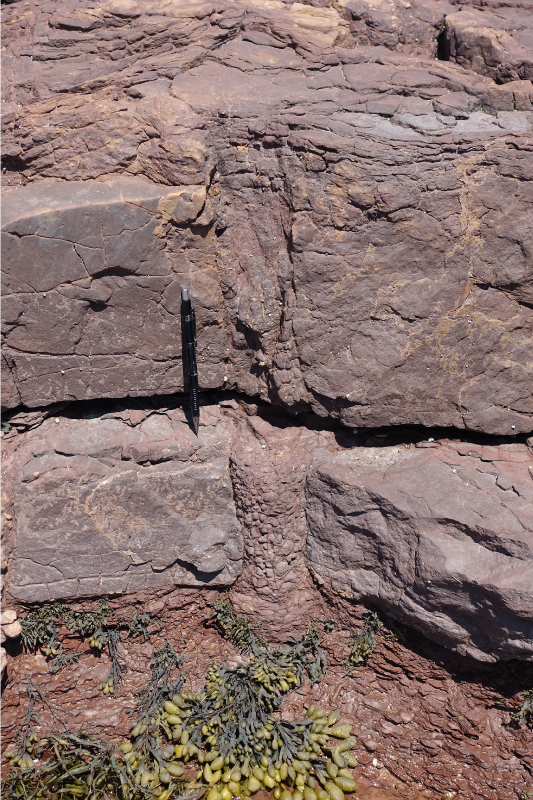
You can read more about Hooke's oolite, and the geological significance of his observations, in an excellent short paper by material scientist Derek Hull (1997). It includes these images of Ketton stone, for comparison with Hooke's drawing:

Reflected light photomicrograph (left) and backscatter scanning electron microscope image (right) of Ketton Stone. Adapted from figures 2 and 3 of Hull (1997). Images are © Royal Society and used in accordance with their terms.

Reflected light photomicrograph (left) and backscatter scanning electron microscope image (right) of Ketton Stone. Adapted from figures 2 and 3 of Hull (1997). Images are © Royal Society and used in accordance with their terms.

I love that this book, which is mostly about the elastic behaviour of rocks, bears an illustration by the man that first described elasticity. Better still, the illustration is of a fractured rock — making it the perfect preface. 


References

Hall, M & E Bianco (eds.) (2016). 52 Things You Should Know About Rock Physics. Nova Scotia: Agile Libre, 134 pp.

Hooke, R (1665). Micrographia: or some Physiological Descriptions of Minute Bodies made by Magnifying Glasses, pp. 93–100. The Royal Society, London, 1665.

Hull, D (1997). Robert Hooke: A fractographic study of Kettering-stone. Notes and Records of the Royal Society of London 51, p 45-55. DOI: 10.1098/rsnr.1997.0005.

52 Things... Rock Physics

There's a new book in the 52 Things family! 

52 Things You Should Know About Rock Physics is out today, and available for purchase at Amazon.com. It will appear in their European stores in the next day or two, and in Canada... well, soon. If you can't wait for that, you can buy the book immediately direct from the printer by following this link.

The book mines the same vein as the previous volumes. In some ways, it's a volume 2 of the original 52 Things... Geophysics book, just a little bit more quantitative. It features a few of the same authors — Sven Treitel, Brian Russell, Rachel Newrick, Per Avseth, and Rob Simm — but most of the 46 authors are new to the project. Here are some of the first-timers' essays:

  • Ludmilla Adam, Why echoes fade.
  • Arthur Cheng, How to catch a shear wave.
  • Peter Duncan, Mapping fractures.
  • Paul Johnson, The astonishing case of non-linear elasticity.
  • Chris Liner, Negative Q.
  • Chris Skelt, Five questions to ask the petrophysicist.

It's our best collection of essays yet. We're very proud of the authors and the collection they've created. It stretches from childhood stories to linear algebra, and from the microscope to seismic data. There's no technical book like it. 

Supporting Geoscientists Without Borders

Purchasing the book will not only bring you profund insights into rock physics — there's more! Every sale sends $2 to Geoscientists Without Borders, the SEG charity that supports the humanitarian application of geoscience in places that need it. Read more about their important work.

It's been an extra big effort to get this book out. The project was completely derailed in 2015, as we — like everyone else — struggled with some existential questions. But we jumped back into it earlier this year, and Kara (the managing editor, and my wife) worked her magic. She loves working with the authors on proofs and so on, but she doesn't want to see any more equations for a while.

If you choose to buy the book, I hope you enjoy it. If you enjoy it, I hope you share it. If you want to share it with a lot of people, get in touch — we can help. Like the other books, the content is open access — so you are free to share and re-use it as you wish. 

Q is for Q

Quality factor, or \(Q\), is one of the more mysterious quantities of seismology. It's right up there with Lamé's \(\lambda\) and Thomsen's \(\gamma\). For one thing, it's wrapped up with the idea of attenuation, and sometimes the terms \(Q\) and 'attenuation' are bandied about seemingly interchangeably. For another thing, people talk about it like it's really important, but it often seems to be completely ignored.

A quick aside. There's another quality factor: the rock quality factor, popular among geomechnicists (geomechanics?). That \(Q\) describes the degree and roughness of jointing in rocks, and is probably related — coincidentally if not theoretically — to seismic \(Q\) in various nonlinear and probably profound ways. I'm not going to say any more about it, but if this interests you, read Nick Barton's book, Rock Quality, Seismic Velocity, Attenuation and Anistropy (2006; CRC Press) if you can afford it. 

So what is Q exactly?

We know intuitively that seismic waves lose energy as they travel through the earth. There are three loss mechanisms: scattering (elastic losses resulting from reflections and diffractions), geometrical spreading, and intrinsic attenuation. This last one, anelastic energy loss due to absorption — essentially the deviation from perfect elasticity — is what I'm trying to describe here.

I'm not going to get very far, by the way. For the full story, start at the seminal review paper entitled \(Q\) by Leon Knopoff (1964), which surely has the shortest title of any paper in geophysics. (Knopoff also liked short abstracts, as you see here.)

The dimensionless seismic quality factor \(Q\) is defined in terms of the energy \(E\) stored in one cycle, and the change in energy — the energy dissipated in various ways, such as fluid movement (AKA 'sloshing', according to Carl Reine's essay in 52 Things... Geophysics) and intergranular frictional heat ('jostling') — over that cycle:

$$ Q \stackrel{\mathrm{def}}{=} 2 \pi \frac{E}{\Delta E} $$

Remarkably, this same definition holds for any resonator, including pendulums and electronics. Physics is awesome!

Because the right-hand side of that relationship is sort of upside down — the loss is in the denominator — it's often easier to talk about \(Q^{-1}\) which is, more or less, the percentage loss of energy in a single wavelength. This inverse of \(Q\) is proportional to the attenuation coefficient. For more details on that relationship, check out Carl Reine's essay.

This connection with wavelengths means that we have to think about frequency. Because high frequencies have shorter cycles (by definition), they attenuate faster than low frequencies. You know this intuitively from hearing the beat, but not the melody, of distant music for example. This effect does not imply that \(Q\) depends on frequency... that's a whole other can of worms. (Confused yet?)

The frequency dependence of \(Q\)

It's thought that \(Q\) is roughly constant with respect to frequency below about 1 Hz, then increases with \(f^\alpha\), where \(\alpha\) is about 0.7, up to at least 25 Hz (I'm reading this in Mirko van der Baan's 2002 paper), and probably beyond. Most people, however, seem to throw their hands up and assume a constant \(Q\) even in the seismic bandwidth... mainly to make life easier when it comes to seismic processing. Attempting to measure, let alone compensate for, \(Q\) in seismic data is, I think it's fair to say, an unsolved problem in exploration geophysics.

Why is it worth solving? I think the main point is that, if we could model and measure it better, it could be a semi-independent measure of some rock properties we care about, especially velocity. Actually, I think it's even a stretch to call velocity a rock property — most people know that velocity depends on frequency, at least across the gulf of frequencies between seismic and acoustic logging tools, but did you know that velocity also depends on amplitude? Paul Johnson tells about this effect in his essay in the forthcoming 52 Things... Rock Physics book — stay tuned for more on that.

For a really wacky story about negative values of \(Q\) — which imply transmission coefficients greater than 1 (think about that) — check out Chris Liner's essay in the same book (or his 2014 paper in The Leading Edge). It's not going to help \(Q\) get any less mysterious, but it's a good story. Here's the punchline from a Jupyter Notebook I made a while back; it follows along with Chris's lovely paper:

Top: Velocity and the Backus average velocity in the E-38 well offshore Nova Scotia. Bottom: Layering-induced attenuation, or 1/Q, in the same well. Note the negative numbers! Reproduction of Liner's 2014 results in a Jupyter Notebook.

Top: Velocity and the Backus average velocity in the E-38 well offshore Nova Scotia. Bottom: Layering-induced attenuation, or 1/Q, in the same well. Note the negative numbers! Reproduction of Liner's 2014 results in a Jupyter Notebook.

Hm, I had hoped to shed some light on \(Q\) in this post, but I seem to have come full circle. Maybe explaining \(Q\) is another unsolved problem.

References

Barton, N (2006). Rock Quality, Seismic Velocity, Attenuation and Anisotropy. Florida, USA: CRC Press. 756 pages. ISBN 9780415394413.

Johnson, P (in press). The astonishing case of non-linear elasticity.  In: Hall, M & E Bianco (eds), 52 Things You Should Know About Rock Physics. Nova Scotia: Agile Libre, 2016, 132 pp.

Knopoff, L (1964). Q. Reviews of Geophysics 2 (4), 625–660. DOI: 10.1029/RG002i004p00625.

Reine, C (2012). Don't ignore seismic attenuation. In: Hall, M & E Bianco (eds), 52 Things You Should Know About Geophysics. Nova Scotia: Agile Libre, 2012, 132 pp.

Liner, C (2014). Long-wave elastic attenuation produced by horizontal layering. The Leading Edge 33 (6), 634–638. DOI: 10.1190/tle33060634.1. Chris also blogged about this article.

Liner, C (in press). Negative Q. In: Hall, M & E Bianco (eds), 52 Things You Should Know About Rock Physics. Nova Scotia: Agile Libre, 2016, 132 pp.

van der Bann, M (2002). Constant Q and a fractal, stratified Earth. Pure and Applied Geophysics 159 (7–8), 1707–1718. DOI: 10.1007/s00024-002-8704-0.

The sound of the Software Underground

If you are a geoscientist or subsurface engineer, and you like computery things — in other words, if you read this blog — I have a treat for you. In fact, I have two! Don't eat them all at once.

Software Underground

Sometimes (usually) we need more diversity in our lives. Other times we just want a soul mate. Or at least someone friendly to ask about that weird new seismic attribute, where to find a Python library for seismic imaging, or how to spell Kirchhoff. Chat rooms are great for those occasions, Slack is where all the cool kids go to chat, and the Software Underground is the Slack chat room for you. 

It's free to join, and everyone is welcome. There are over 130 of us in there right now — you probably know some of us already (apart from me, obvsly). Just go to http://swung.rocks/ to sign up, and we will welcome you at the door with your choice of beverage.

To give you a flavour of what goes on in there, here's a listing of the active channels:

  • #python — for people developing in Python
  • #sharp-rocks — for people developing in C# or .NET
  • #open-geoscience — for chat about open access content, open data, and open source software
  • #machinelearning — for those who are into artificial intelligence
  • #busdev — collaboration, subcontracting, and other business opportunities 
  • #general — chat about anything to do with geoscience and/or computers
  • #random — everything else

Undersampled Radio

If you have a long commute, or occasionally enjoy being trapped in an aeroplane while it flies around, you might have discovered the joy of audiobooks and podcasts. You've probably wished many times for a geosciencey sort of podcast, the kind where two ill-qualified buffoons interview hyper-intelligent mega-geoscientists about their exploits. I know I have.

Well, wish no more because Undersampled Radio is here! Well, here:

The show is hosted by New Orleans-based geophysicist Graham Ganssle and me. Don't worry, it's usually not just us — we talk to awesome guests like geophysicists Mika McKinnon and Maitri Erwin, geologist Chris Jackson, and geopressure guy Mark Tingay. The podcast is recorded live every week or three in Google Hangouts on Air — the link to that, and to show notes and everything else — is posted by Gram in the #undersampled Software Underground channel. You see? All these things are connected, albeit in a nonlinear, organic, highly improbable way. Pseudoconnection: the best kind of connection.

Indeed, there is another podcast pseudoconnected to Software Underground: the wonderful Don't Panic Geocast — hosted by John Leeman and Shannon Dulin — also has a channel: #dontpanic. Give their show a listen too! In fact, here's a show we recorded together!

Don't have an hour right now? OK, you asked for it, here's a clip from that show to get you started. It starts with John Leeman explaining what Fun Paper Friday is, and moves on to one of my regular rants about conferences...

In case you're wondering, neither of these projects is explicitly connected to Agile — I am just involved in both of them. I just wanted to clear up any confusion. Agile is not a podcast company, for the time being anyway.

In search of the Kennetcook Thrust

Behind every geologic map, is a much more complex geologic truth. Most of the time it's hidden under soil and vegetation, forcing geologists into a detective game in order to fill gaps between hopelessly sparse spatterings of evidence.

Two weeks ago, I joined up with an assortment of geologists on the side of the highway an hour north of Halifax for John Waldron to guide us along some spectacular stratigraphy exposed in the coastline cliffs on the southern side of the Minas Basin (below). John has visited these sites repeatedly over his career, and he's supervised more than a handful of graduate students probing a variety of geologic processes on display here. He's published numerous papers teasing out the complex evolution of the Windsor-Kennetcook Basin: one of three small basins onshore Nova Scotia with the potential to contain economic quantities of hydrocarbons.

John retold the history of mappers past and present riddled by the massively deformed, often duplicated Carboniferous evaporites in the Windsor Group which are underlain by sub-horizontal seismic reflectors at depth. Local geologists agree that this relationship reflects thrusting of the near-surface package, but there is disagreement on where this thrust is located, and whether and where it intersects the surface. On this field trip, John showed us symptoms of this Kennetcook thrust system, at three sites. We started in the footwall. The second and third sites were long stretches spectacularly deformed exposures in the hangingwall.  

Footwall: Cheverie Point

SEE GALLERY BELOW FOR ENLARGEMENT

SEE GALLERY BELOW FOR ENLARGEMENT

The first stop was Cheverie Point and is interpreted to be well in the footwall of the Kennetcook thrust. Small thrust faults (right) cut through the type section of the Macumber Formation and match the general direction of the main thrust system. The Macumber Formation is a shallow marine microbial limestone that would have fooled anyone as a mudstone, except it fizzed violently under a drop of HCl. Just to the right of this photo, we stood on the unconformity between the petroliferous and prospective Horton Group and the overlying Windsor Group. It's a pick that turns out to be one of the most reliably mappable seismic events on seismic sections so it was neat to stand on that interface.

Further down section we studied the Mississippian Cheverie Formation: stacked cycles of point-bar deposits ranging from accretionary lag conglomerates to caliche paleosols with upright tree trunks. Trees more than a metre or more in diameter were around from the mid Devonian, but Cheverie forests are still early and good examples of trees within point-bars and levees.  

Hangingwall: Red Head / Johnson Beach / Split Rock

SEE GALLERY BELOW FOR ENLARGEMENT

SEE GALLERY BELOW FOR ENLARGEMENT

The second site featured some spectacularly folded black shales from the Horton Bluff Formation, as well as protruding sills up to two metres thick that occasionally jumped across bedding (right). We were clumsily contemplating the curious occurrence of these intrusions for quite some time until hard-rock guru Trevor McHattie halted the chatter, struck off a clean piece rock with a few blows of his hammer, wetted it with a slobbering lick, and inspected it with his hand lens. We all watched him in silence and waited for his description. I felt a little schooled. He could have said anything. It was my favourite part of the day.

Hangingwall continued: Rainy Cove

The patterns in the rocks at Rainy Cove are a wonderland for any structural geologist. It's a popular site for geology labs from Atlantic Universities, but it would be an absolute nightmare to try to actually measure the section here. 

SEE GALLERY BELOW FOR ENLARGEMENT

SEE GALLERY BELOW FOR ENLARGEMENT

John stands next to a small system of duplicated thrusts in the main hangingwall that have been subsequently folded (left). I tried tracing out the fault planes by following the offsets in the red sandstone bed amidst black shales whose fabric has been deformed into an accordion effect. Your picks might very well be different from mine.

A short distance away we were pointed to an upside-down view of load structures in folded beds. "This antiform is a syncline", John paused while we processed. "This synform over here is an anticline". Features telling of such intense deformation are hard to fathom. Especially in plain sight.

The rock lessons ended in the early evening at the far end of Rainy Cove where the Triassic Wolfville formation sits unconformably on top of ridiculously folded, sometimes doubly overturned Carboniferous Horton Rocks. John said it has to be one of the most spectacularly exposed unconformities in the world. 

I often take for granted the vast stretches of geology hiding beneath soil and vegetation, and the preciousness of finding quality outcrop. Check out the gallery below for pictures from our day.  

I was quite enamoured with John's format. His field trip technologies. The maps and sections: canvases for communication and works in progress. His white boarding, his map-folding techniques: a practised impresario.

What are some of the key elements from the best field trips you've been on? Let us know in the comments.

Automated interpretation highlights

As you probably know by know, I've been at the EAGE conference in Vienna this week. I skipped out yesterday and flew over to the UK for a few days. I have already written plenty about the open source workshop, and I will write more soon about the hackathon. But I thought I'd pass on my highlights from the the Automated Interpretation session on Tuesday. In light of Monday's discussion, I made a little bit of a nuisance of myself by asking the same post-paper question every time I got the chance:

Can I use your code, either commercially or for free?

I'll tell you what the authors responded.


The universal character of salt

I especially enjoyed the presentation by Anders Waldeland and Anne Solberg (University of Oslo) on automatically detecting salt in 3D seismic. (We've reported on Anne Solberg's work before.) Anders described training eight different classifiers, from a simple nearest mean to a neural network, a supprt vector model, and a mixture of Gaussians classifier. Interestingly, but not surprisingly, the simplest model turned out to be the most effective at discrimination. He also tried a great many seismic attributes, letting the model choose the best ones. Three attributes consistently proved most useful: coherency, Haralick energy (a GLCM-based texture attribute), and the variance of the kurtosis of the amplitude distribution (how's that for meta?). What was especially interesting about his approach was that he was training the models on one dataset, and predicting on an entirely different 3D. The idea is that this might reveal the universal seismic characteristics of salt. When I asked the golden question, he said "Come and talk to me", which isn't a "yes", but it isn't a "no" either.

Waldeland and Solberg 2016. Salt probability in a North Sea dataset (left) and the fully tracked volume (right). The prediction model was trained on a Gulf of Mexico dataset. Copyright of the authors and EAGE, and used under a Fair Use claim.

Waldeland and Solberg 2016. Salt probability in a North Sea dataset (left) and the fully tracked volume (right). The prediction model was trained on a Gulf of Mexico dataset. Copyright of the authors and EAGE, and used under a Fair Use claim.

Secret horizon tracker

Horizons tracked with Figueiredo et al's machine learning algorithm. The horizons correctly capture the discontinuities. Copyright of the authors and EAGE. Used under a Fair Use claim.

Horizons tracked with Figueiredo et al's machine learning algorithm. The horizons correctly capture the discontinuities. Copyright of the authors and EAGE. Used under a Fair Use claim.

The most substantial piece of machine learning I saw was Eduardo Figueiredo from Pontifical Catholic University in Rio, in the same session as Waldeland. He's using a neural net called Growing Neural Gas to classify (aka or 'label') the input data in a number of different ways. This training step takes a little time. The label sets can now be compared to decide on the similarity between two samples, based on the number of labels the samples have in common but also including a comparison to the original seed, which essentially acts as a sort of brake to stop things running away. This progresses the pick. If a decision can't be reached, a new global seed is selected randomly. If that doesn't work, picking stops. Unfortunately he did not show a comparison to an ordinary autotracker, either in terms of time or quality, but the results did look quite good. The work was done 'in cooperation with Petrobras', so it's not surprising the code is not available. I was a bit surprised that Figueiredo was even unable to share any details of the implementation.

More on interpretation

The other two interesting talks in the session were two from Paul de Groot (dGB Earth Sciences) and Gaynor Paton (GeoTeric). Paul introduced the new Thalweg Tracker in OpendTect — the only piece of software from the session that you can actually run, albeit for a fee — which is a sort of conservative voxel tracker. Unsurprisingly, Paul was also very thorough with his examples, and his talk served as a tutorial in how to make use of, and give attribution to, open data. (I'm nearly done with the grumbling about openness for now, I promise, but I can't help mentioning that I find it a bit ironic that those scientists unwilling to share their work are also often a bit lax with giving credit to others whose work they depend on.)

Gaynor's talk was about colour, which you may know we enjoy thinking about. She had gathered 24 seismic interpreters, five of whom had some form of colour deficiency. She gave the group some interpretation tasks, and tried to gauge their performance in the tasks. It seemed interesting enough, and I immediately wondered if we could help out with Pick This, especially to help grow the sample size, and by blinding the study. But the conclusion seemed to be that, if there are ways in which colour blind interpreters are less capable at image interpretation, for example where hue is important, they compensate for it by interpreting other aspects, such as contrast and shape. 

Paton's research into how colour deficient people interpret attributes. There were 5 colour deficient subjects and 19 colour normal. The colour deficient subjects were more senstive to subtle changes in saturation and to feature shapes. Image c…

Paton's research into how colour deficient people interpret attributes. There were 5 colour deficient subjects and 19 colour normal. The colour deficient subjects were more senstive to subtle changes in saturation and to feature shapes. Image copyright Paton and EAGE, and used here under a fair use claim.

That's it for now. I have a few other highlights to share; I'll try to get to them next week. There was a bit of buzz around the Seismic Apparition talks from ETHZ and Statoil, for example. If you were at the conference, I'd love to hear your highlights too, please share them in the comments.

References

A.U. Waldeland* (University of Oslo) & A.H.S. Solberg (University of Oslo). 3D Attributes and Classification of Salt Bodies on Unlabelled Datasets. 78th EAGE Conference & Exhibition 2016. DOI 10.3997/2214-4609.201600880. Available in EarthDoc.

M. Pelissier (Dagang Zhaodong Oil Company), C. Yu (Dagang Zhaodong Oil Company), R. Singh (dGB Earth Sciences), F. Qayyum (dGB Earth Sciences), P. de Groot* (dGB Earth Sciences) & V. Romanova (dGB Earth Sciences). Thalweg Tracker - A Voxel-based Auto-tracker to Map Channels and Associated Margins. 78th EAGE Conference & Exhibition 2016. DOI 10.3997/2214-4609.201600879. Available in EarthDoc. 

G. Paton* (GeoTeric). The Effect of Colour Blindness on Seismic Interpretation. 78th EAGE Conference & Exhibition 2016. DOI 10.3997/2214-4609.201600883. Available in EarthDoc.

A.M. Figueiredo* (Tecgraf / PUC-Rio), J.P. Peçanha (Tecgraf / PUC-Rio), G.M. Faustino (Tecgraf / PUC-Rio), P.M. Silva (Tecgraf / PUC-Rio) & M. Gattass (Tecgraf / PUC-Rio). High Quality Horizon Mapping Using Clustering Algorithms. 78th EAGE Conference & Exhibition 2016. DOI 10.3997/2214-4609.201600878. Available in EarthDoc.

Poisson's controversial stretch-squeeze ratio

Before reading this, you might want to check out the previous post about Siméon Denis Poisson's life and career. Then come back here...


Physicists and mathematicians knew about Poisson's ratio well before Poisson got involved with it. Thomas Young described it in his 1807 Lectures on Natural Philosophy and the Mechanical Arts:

We may easily observe that if we compress a piece of elastic gum in any direction, it extends itself in other directions: if we extend it in length, its breadth and thickness are diminished.

Young didn't venture into a rigorous formal definition, and it was referred to simply as the 'stretch-squeeze ratio'.

A new elastic constant?

Twenty years later, at a time when France's scientific muscle was fading along with the reign of Napoleon, Poisson published a paper attempting to restore his slightly bruised (by his standards) reputation in the mechanics of physical materials. In it, he stated that for a solid composed of molecules tightly held together by central forces on a crystalline lattice, the stretch squeeze ratio should equal 1/2 (which is equivalent to what we now call a Poisson's ratio of 1/4). In other words, Poisson regarded the stretch-squeeze ratio as a physical constant: the same value for all solids, claiming, 'This result agrees perfectly' with an experiment that one of his colleagues, Charles Cagniard de la Tour, recently performed on brass. 

Poisson's whole-hearted subscription to the corpuscular school certainly prejudiced his work. But the notion of discovering of a new physical constant, like Newton did for gravity, or Einstein would eventually do for light, must have been a powerful driving force. A would-be singular elastic constant could unify calculations for materials soft or stiff — in contrast to elastic moduli which vary over several orders of magnitude. 

Poisson's (silly) ratio

Later, between 1850 and 1870, the physics community acquired more evidence that the stretch-squeeze ratio was different for different materials, as other materials were deformed with more reliable measurements. Worse still, de la Tour's experiments on the elasticity of brass, upon which Poisson had hung his hat, turned out to be flawed. The stretch-squeeze ratio became known as Poisson's ratio not as a tribute to Poisson, but as a way of labeling a flawed theory. Indeed, the falsehood became so apparent that it drove the scientific community towards treating elastic materials as continuous media, as opposed to an ensemble of particles.

Today we define Poisson's ratio in terms of strain (deformation), or Lamé's parameters, or the speed \(V\) of P- and S-waves:


Interestingly, if Poisson turned out to be correct, and Poisson's ratio was in fact a constant, that would mean that the number of elastic constants it would take to describe an isotropic material would be one instead of two. It wasn't until Augustin Louis Cauchy used the notion of a stress tensor to describe the state of stress at a point within a material, with its three normal stresses and three shear stresses, did the need for two elastic constants become apparent. Tensors gave the mathematical framework to define Hooke's law in three dimensions. Found in the opening chapter in any modern textbook on seismology or mechanical engineering, continuum mechanics represents a unique advancement in science set out to undo Poisson's famously false deductions backed by insufficient data.

References

Greaves, N (2013). Poisson's ratio over two centuries: challenging hypothesis. Notes & Records of the Royal Society 67, 37-58. DOI: 10.1098/rsnr.2012.0021

Editorial (2011). Poisson's ratio at 200, Nature Materials10 (11) Available online.


Great geophysicists #13: Poisson

Siméon Denis Poisson was born in Pithiviers, France, on 21 June 1781. While still a teenager, Poisson entered the prestigious École Polytechnique in Paris, and published his first papers in 1800. He was immediately befriended — or adopted, really — by Lagrange and Laplace. So it's safe to say that he got off to a pretty good start as a mathematician. The meteoric trajectory continued throughout his career, as Poisson received more or less every honour a French scientist could accumulate. Along with Laplace and Lagrange — as well as Fresnel, Coulomb, Lamé, and Fourier — his is one of the 72 names on the Eiffel Tower.

Wrong Poisson

In the first few decades following the French Revolution, which ended in 1799, France enjoyed a golden age of science. The Société d’Acrueil was a regular meeting of savants, hosted by Laplace and the chemist Claude Louis Berthollet, and dedicated to the exposition of physical phenomena. The group worked on problems like the behaviour of gases, the physics of sound and light, and the mechanics of deformable materials. Using Newton's then 120-year-old law of gravitation as an analogy, the prevailing school of thought accounted for all physical phenomena in terms of forces acting between particles. 

Poisson was not flawless. As one of the members of this intellectual inner circle, Poisson was devoted to the corpuscular theory of light. Indeed, he dismissed the wave theory of light completely, until proven wrong by Thomas Young and, most conspicuously, Augustin-Jean Fresnel. Even Poisson's ratio, the eponymous elastic modulus, wasn't the result of his dogged search for truth, but instead represents a controversy that drove the development of the three-dimensional theory of elasticity. More on this next time.

The workaholic

Although he did make time for his wife and four children — but only after 6 pm — Poisson apparently had little time for much besides mathematics. His catchphrase was

Life is only good for two things: doing mathematics and teaching it.

In the summer of 1838, he learned he had a form of tuberculosis. According to James (2002), he was unable to take time away from work for long enough to recuperate. Eventually, insisting on conducting the final exams at the Polytechnique for the 23rd year in a row, he took on more than he could handle. He died on 20 April 1840. 


References

Grattan-Guinness, I. (1990). Convolutions in French Mathematics, 1800-1840: From the Calculus and Mechanics to Mathematical Analysis and Mathematical Physics. Vol.1: The Setting. Springer Science & Business Media. 549 pages.

Ioan James, I (2002). Remarkable Mathematicians: From Euler to Von Neumann. Cambridge University Press, 433 pages.

The University of St Andrews MacTutor archive article on Poisson.

Deriving equations in Python

Last week I wrote about the elastic moduli, and showed the latest version of my table of equations. Here it is; click on it for a large version:

Making this grid was a bit of an exercise in itself. One could spend some happy hours rearranging things by hand; instead, I spent some (mostly) happy hours learning to use SymPy, a symbolic maths library for Python. For what it's worth, you can see my flailing in this Jupyter Notebook. Warning: it's pretty untidy.

Wrangling equations

Fortunately, SymPy is easy to get started with. Let's look at getting an expression for \(V_\mathrm{P}\) in terms of \(E\) and \(K\), given that I already have an expression in terms of \(E\) and \(\mu\), plus an expression for \(\mu\) in terms of \(E\) and \(K\).

First we import the SymPy library, set it up for nice math display in the Notebook, and initialize some parameter names:

 
>>> import sympy
>>> sympy.init_printing(use_latex='mathjax')
>>> lamda, mu, nu, E, K, rho = sympy.symbols("lamda, mu, nu, E, K, rho")

lamda is not a typo: lambda means something else in Python — it's a sort of unnamed function.

Now we're ready to define an expression. First, I'll import SymPy's own square root function for convenience. Then I define an expression for \(V_\mathrm{P}\) in terms of \(E\) and \(\mu\):

 
>>> vp_expr = sympy.sqrt((mu * (E - 4*mu)) / (rho * (E - 3*mu)))
>>> vp_expr

$$ \sqrt{\frac{\mu \left(E - 4 \mu\right)}{\rho \left(E - 3 \mu\right)}} $$

Now we can give SymPy the expression for \(\mu\) in terms of \(E\) and \(K\) and substitute:

 
>>> mu_expr = (3 * K * E) / (9 * K - E)
>>> vp_new = vp_expr.subs(mu, mu_expr)
>>> vp_new

$$\sqrt{3} \sqrt{\frac{E K \left(- \frac{12 E K}{- E + 9 K} + E\right)}{\rho \left(- E + 9 K\right) \left(- \frac{9 E K}{- E + 9 K} + E\right)}}$$

Argh, what is that?? Luckily, it's easy to simplify:

 
>>> sympy.simplify(vp_new)

$$\sqrt{3} \sqrt{\frac{K \left(E + 3 K\right)}{\rho \left(- E + 9 K\right)}}$$

That's more like it! What's really cool is that SymPy can even generate the \(\LaTeX\) code for your favourite math renderer:

 
>>> print(sympy.latex(sympy.simplify(vp_new)))
\sqrt{3} \sqrt{\frac{K \left(E + 3 K\right)}{\rho \left(- E + 9 K\right)}}

That's all there is to it!

What is the mystery X?

Have a look at the expression for  \(V_\mathrm{P}\) in terms of \(E\) and \(\lambda\):


$$\frac{\sqrt{2}}{2} \sqrt{\frac{1}{\rho} \left(E - \lambda + \sqrt{E^{2} + 2 E \lambda + 9 \lambda^{2}}\right)}$$

I find this quantity — I call it \(X\) in the big table of equations — really curious:


$$ X = \sqrt{9\lambda^2 + 2E\lambda + E^2} $$

As you can see from the similar table on Wikipedia, a similar quantity appears in expressions in terms of \(E\) and \(M\). These quantities look like elastic moduli, and even have the right units and order of magnitude as the others. If anyone has thoughts on what significance it might have, if any, or on why expressions in terms of \(E\) and \(\lambda\) or \(M\) should be so uncommonly clunky, I'm all ears. 

One last thing... I've mentioned Melvyn Bragg's wonderful BBC radio programme In Our Time before. If you like listening to the radio, try this recent episode on the life and work of Robert Hooke. Not only did he invent the study of elasticity with his eponymous law, he was also big in microscopy, describing things like the cellular structure of cork in detail (right).

All the elastic moduli

An elastic modulus is the ratio of stress (pressure) to strain (deformation) in an isotropic, homogeneous elastic material:

$$ \mathrm{modulus} = \frac{\mathrm{stress}}{\mathrm{strain}} $$

OK, what does that mean?

Elastic means what you think it means: you can deform it, and it springs back when you let go. Imagine stretching a block of rubber, like the picture here. If you measure the stress \(F/W^2\) (i.e. the pressure is force per unit of cross-sectional area) and strain \(\Delta L/L\) (the stretch as a proportion) along the direction of stretch ('longitudinally'), then the stress/strain ratio gives you Young's modulus, \(E\).

Since strain is unitless, all the elastic moduli have units of pressure (pascals, Pa), and is usually on the order of tens of GPa (billions of pascals) for rocks. 

The other elastic moduli are: 

There's another quantity that doesn't fit our definition of a modulus, and doesn't have units of pressure — in fact it's unitless —  but is always lumped in with the others: 

What does this have to do with my data?

Interestingly, and usefully, the elastic properties of isotropic materials are described completely by any two moduli. This means that, given any two, we can compute all of the others. More usefully still, we can also relate them to \(V_\mathrm{P}\), \(V_\mathrm{S}\), and \(\rho\). This is great because we can get at those properties easily via well logs and less easily via seismic data. So we have a direct path from routine data to the full suite of elastic properties.

The only way to measure the elastic moduli themselves is on a mechanical press in the laboratory. The rock sample can be subjected to confining pressures, then squeezed or stretched along one or more axes. There are two ways to get at the moduli:

  1. Directly, via measurements of stress and strain, so called static conditions.

  2. Indirectly, via sonic measurements and the density of the sample. Because of the oscillatory and transient nature of the sonic pulses, we call these dynamic measurements. In principle, these should be the most comparable to the measurements we make from well logs or seismic data.

Let's see the equations then

The elegance of the relationships varies quite a bit. Shear modulus \(\mu\) is just \(\rho V_\mathrm{S}^2\), but Young's modulus is not so pretty:

$$ E = \frac{\rho V_\mathrm{S}^2 (3 V_\mathrm{P}^2 - 4 V_\mathrm{S}^2) }{V_\mathrm{P}^2 - V_\mathrm{S}^2} $$

You can see most of the other relationships in this big giant grid I've been slowly chipping away at for ages. Some of it is shown below. It doesn't have most of the P-wave modulus expressions, because no-one seems too bothered about P-wave modulus, despite its obvious resemblance to acoustic impedance. They are in the version on Wikipedia, however (but it lacks the \(V_\mathrm{P}\) and \(V_\mathrm{S}\) expressions).

Some of the expressions for the elastic moduli and velocities — click the image to see them all in SubSurfWiki.

Some of the expressions for the elastic moduli and velocities — click the image to see them all in SubSurfWiki.

In this table, the mysterious quantity \(X\) is given by:

$$ X = \sqrt{9\lambda^2 + 2E\lambda + E^2} $$

In the next post, I'll come back to this grid and tell you how I've been deriving all these equations using Python.


Top tip... To find more posts on rock physics, click the Rock Physics tag below!