Are there benefits to pseudoscience?

No, of course there aren't. 

Balance! The scourge of modern news. CC-BY by SkepticalScience.com

Balance! The scourge of modern news. CC-BY by SkepticalScience.com

Unless... unless you're a journalist, perhaps. Then a bit of pseudoscience can provide some much-needed balance — just to be fair! — to the monotonic barrage of boring old scientific consensus. Now you can write stories about flat-earthers, anti-vaxxers, homeopathy, or the benefits of climate change!*

So far, so good. It's fun to pillory the dimwits who think the moon landings were filmed in a studio in Utah, or that humans have had no impact on Earth's climate. The important thing is for the journalist to have a clear and unequivocal opinion about it. If an article doesn't make it clear that the deluded people at the flat-earth convention ("Hey, everyone thought Copernicus was mad!") have formed their opinions in spite of, not because of, the overwhelming evidence before them, then readers might think the journalist — and the publisher — agree with them.

In other words, if you report on hogwash, then you had better say that it's hogwash, or you end up looking like one of the washers of the hog.


Fake geoscience?

AAPG found this out recently, when the August issue of its Explorer magazine published an article by Ken Milam called Are there benefits to climate change? Ken was reporting on a talk by AAPG member Greg Wrightstone at URTeC in July. Greg wrote a book called Inconvenient Facts: The Science That Al Gore Doesn't Want You To Know. The gist: no need to be concerned about carbon dioxide because, "The U.S. Navy’s submarines often exceed 8,000 ppm (20 times current levels) and there is no danger to our sailors" — surely some of the least watertight reasoning I've ever encountered. Greg's basic idea is that, since the earth has been warmer before, with higher levels of CO2, there's nothing to worry about today (those Cretaceous conurbations and Silurian civilizations had no trouble adapting!) So he thinks, "the correct policy to address climate change is to have the courage to do nothing".

So far, so good. Except that Ken — in reporting 'just the facts' — didn't mention that Greg's talk was full of half-truths and inaccuracies and that few earth scientists agree with him. He forgot to remark upon the real news story: how worrying it is that URTeC 2018 put on a breakfast promoting Greg and his marginal views. He omitted to point out that this industry needs to grow up and face the future with reponsibility, supporting society with sound geoscience.

So it looked a bit like Explorer and AAPG were contributing to the washing of this particular hog.


Discussion

As you might expect, there was some discussion about the article — both on aapg.org and on Twitter (and probably elsewhere). For example, Mark Tingay (University of Adelaide) called AAPG and SPE out:

So did Brian Romans (Virginia Tech):

And there was further discussion (sort of) involving Greg Wrightstone himself. Trawl through Mark Tingay's timeline, especially his systematic dismantling of Greg's 'evidence', if your curiosity gets the better of you.


Response

Of course AAPG noticed the commotion. The September issue of Explorer contains two statements from AAPG staff. David Curtiss, AAPG Executive Director, said this in his column:

Milam was assigned to report on an invited presentation by Greg Wrightstone, a past president of AAPG’s Eastern Section, based on a recently self-published book on climate change, at the Unconventional Resources Technology Conference in July. Here was an AAPG Member and past section officer speaking about climate change – an issue of interest to many of our members, who had been invited by a group of his geoscience and engineering peers to present at a topical breakfast – not a technical session – at a major conference.

This sounds fine, on the face of it, but details matter. A glance at the book in question should have been enough to indicate that the content of the talk could only have been presented in a non-technical session, with a side of hash browns.

Anyway, David does go on to point out the tension between the petroleum industry's activities and society's environmental concerns. The tension is real, and AAPG and its members, are in the middle of it. We can contribute scientifically to the conversations that need to happen to resolve that tension. But pushing junk science and polemical bluster is definitely not going to help. I believe that most of the officers and members of AAPG agree. 

The editor of Explorer, Brian Ervin, had this to say:

For the record, none of our coverage of any issue or any given perspective on an issue should be taken as an endorsement — explicit or implicit — of that perspective. Also, the EXPLORER is — quite emphatically — not a scientific journal. Our content is not peer-reviewed. [...] No, the EXPLORER exists for an entirely different purpose. We provide news about Earth science, the industry and the Association, so our mission is different and unrelated to that of a scientific publication.

He goes on to say that he knew that Wrightstone's views are not popular and that it would provoke some reaction, but wanted to present it impartially and "give [readers] the opportunity to evaluate his position for themselves".

I just hope Explorer doesn't start doing this with too many other marginal opinions.


I'd have preferred to see AAPG back-pedal a bit more energetically. Publishing this article was a mistake. AAPG needs to think about the purpose, and influence, of its reporting, as well as its stance on climate change (which, according to David Curtiss, hasn't been discussed substantially in more than 10 years). This isn't about pushing agendas, any more than talking about the moon landings is about pushing agendas. It's about being a modern scientific association with high aspirations for itself, its members, and society.

Get out of the way

This tweet from the Ecological Society of America conference was interesting:

This kind of thing is not new — many conferences have 'No photos' signs around the posters and the talk sessions. 'No tweeting' seems pretty extreme though. I'm not sure if that's what the ESA was pushing for in this case, but either way the message is: 'No sharing stuff'. They do have a hashtag though, so...

Anyway, I tweeted this in response:

I think this tells you just as much about how broken the conference model is, as about how naïve/afraid our technical societies are.

I think there's a general rule: if you're trying to control the flow of information, you're getting in the way. You're also going to be disappointed because you can't control the flow of information — perhaps because it's not yours to control. I want to say to the organizers: The people you invited into your society are, thankfully, enthusiastic collaborators who can't wait to share the exciting things they heard at your conference. Why on earth would you try to shut that down? Why wouldn't you go out of your way to support them, amplify them, and find more people like them?

But wait, the no-tweeting society asks, what if the author didn't want anyone to share their work? My first question is: why did you give a talk then? My second question is: did the sharer give you proper attribution? If not — you are right to be annoyed and your society should help set this norm in your community. If so — see my first question.

Technical societies need to get over the idea that they own their communities and the knowledge their communities produce. They fret about revenue and membership numbers, but they just need to focus on making their members' technical and professional lives richer and more connected. The rest will take care of itself.


Interested in this topic? Here's a great post about tweeting at conferences, by Jacquelyn Gill. It also links to lots of other opinions, and there are lots of comments.

Image by Rob Salguero-Gómez.

It's Dynamic Range Day!

OK signal processing nerds, which side are you on in the Loudness War?

If you haven't heard of the Loudness War, you have some catching up to do! This little video by Matt Mayfield is kinda low-res but it's the shortest and best explanation I've been able to find. Watch it, then choose sides >>>>

There's a similar-but-slightly-different war going on in photography: high-dynamic-range or HDR photography is, according to some purists, an existential threat to photography. I'm not going to say any more about it today, but these HDR disasters speak volumes.

True amplitudes

The ideology at the heart of the Loudness War is that music production should be 'pure'. It's analogous to the notion that amplitudes in seismic images should be 'true', and just as nuanced. For some, the idea could be to get as close as possible to a live performance, for others it might be to create a completely synthetic auditory experience; for a record company the main point is to be noticed and then purchased (or at least searched for on Spotify). It reminds me a bit of the aesthetically

For a couple of decades, mainstream producers succumbed to the misconception that driving up the loudness — by increasing the mean amplitude, in turn by reducing the peaks and boosting the quiet passages — was the solution. But this seems to be changing. Through his tireless dedication to the cause, engineer Ian Shepherd has been a key figure in unpeeling this idée fixe. As part of his campaigning, he instituted Dynamic Range Day, and tomorrow is the 8th edition. 

If you want to hear examples of well-produced, dynamic music, check out the previous winners and runners up of the Dynamic Range Day Award — including tunes by Daft Punk, The XX, Kendrick Lamar, and at the risk of dating myself, Orbital.

The end is in sight

I'll warn you right now — this Loudness War thing is a bit of a YouTube rabbithole. But if you still haven't had enough, it's worth listening to the legendary Bob Katz talking about the weapons of war.

My takeaway: the war is not over, but battles are being won. For example, Spotify last year reduced its target output levels, encouraging producers to make more dynamic records. Katz ends his video with "2020 will be like 1980" — which is a good thing, in terms of audio engineering — and most people seem to think the Loudness War will be over.

Real and apparent seismic frequency

There's a Jupyter Notebook for you to follow along with this tutorial. You can run it right here in your browser.


We often use Ricker wavelets to model seismic, for example when making a synthetic seismogram with which to help tie a well. One simple way to guesstimate the peak or central frequency of the wavelet that will model a particlar seismic section is to count the peaks per unit time in the seismic. But this tends to overestimate the actual frequency because the maximum frequency of a Ricker wavelet is more than the peak frequency. The question is, how much more?

To investigate, let's make a Ricker wavelet and see what it looks like in the time and frequency domains.

>>> T, dt, f = 0.256, 0.001, 25

>>> import bruges
>>> w, t = bruges.filters.ricker(T, dt, f, return_t=True)

>>> import scipy.signal
>>> f_W, W = scipy.signal.welch(w, fs=1/dt, nperseg=256)
The_frequency_of_a_Ricker_2_0.png

When we count the peaks in a section, the assumption is that this apparent frequency — that is, the reciprocal of apparent period or distance between the extrema — tells us the dominant or peak frequency.

To help see why this assumption is wrong, let's compare the Ricker with a signal whose apparent frequency does match its peak frequency: a pure cosine:

>>> c = np.cos(2 * 25 * np.pi * t)
>>> f_C, C = scipy.signal.welch(c, fs=1/dt, nperseg=256)
The_frequency_of_a_Ricker_4_0.png

Notice that the signal is much narrower in bandwidth. If we allowed more oscillations, it would be even narrower. If it lasted forever, it would be a spike in the frequency domain.

Let's overlay the signals to get a picture of the difference in the relative periods:

The_frequency_of_a_Ricker_6_1.png

The practical consequence of this is that if we estimate the peak frequency to be \(f\ \mathrm{Hz}\), then we need to reduce \(f\) by some factor if we want to design a wavelet to match the data. To get this factor, we need to know the apparent period of the Ricker function, as given by the time difference between the two minima.

Let's look at a couple of different ways to find those minima: numerically and analytically.

Find minima numerically

We'll use scipy.optimize.minimize to find a numerical solution. In order to use it, we'll need a slightly different expression for the Ricker function — casting it in terms of a time basis t. We'll also keep f as a variable, rather than hard-coding it in the expression, to give us the flexibility of computing the minima for different values of f.

Here's the equation we're implementing:

$$ w(t, f) = (1 - 2\pi^2 f^2 t^2)\ e^{-\pi^2 f^2 t^2} $$

In Python:

>>> def ricker(t, f):
>>>     return (1 - 2*(np.pi*f*t)**2) * np.exp(-(np.pi*f*t)**2)

Check that the wavelet looks like it did before, by comparing the output of this function when f is 25 with the wavelet w we were using before:

>>> f = 25
>>> np.allclose(w, ricker(t, f=25))
True

Now we call SciPy's minimize function on our ricker function. It itertively searches for a minimum solution, then gives us the x (which is really t in our case) at that minimum:

>>> import scipy.optimize
>>> f = 25
>>> scipy.optimize.minimize(ricker, x0=0, args=(f))

fun: -0.4462603202963996
 hess_inv: array([[1]])
      jac: array([-2.19792128e-07])
  message: 'Optimization terminated successfully.'
     nfev: 30
      nit: 1
     njev: 10
   status: 0
  success: True
        x: array([0.01559393])

So the minimum amplitude, given by fun, is -0.44626 and it occurs at an x (time) of \(\pm 0.01559\ \mathrm{s}\).

In comparison, the minima of the cosine function occur at a time of \(\pm 0.02\ \mathrm{s}\). In other words, the period appears to be \(0.02 - 0.01559 = 0.00441\ \mathrm{s}\) shorter than the pure waveform, which is...

>>> (0.02 - 0.01559) / 0.02
0.22050000000000003

...about 22% shorter. This means that if we naively estimate frequency by counting peaks or zero crossings, we'll tend to overestimate the peak frequency of the wavelet by about 22% — assuming it is approximately Ricker-like; if it isn't we can use the same method to estimate the error for other functions.

This is good to know, but it would be interesting to know if this parameter depends on frequency, and also to have a more precise way to describe it than a decimal. To get at these questions, we need an analytic solution.

Find minima analytically

Python's SymPy package is a bit like Maple — it understands math symbolically. We'll use sympy.solve to find an analytic solution. It turns out that it needs the Ricker function writing in yet another way, using SymPy symbols and expressions for \(\mathrm{e}\) and \(\pi\).

import sympy as sp
t, f = sp.Symbol('t'), sp.Symbol('f')
r = (1 - 2*(sp.pi*f*t)**2) * sp.exp(-(sp.pi*f*t)**2)

Now we can easily find the solutions to the Ricker equation, that is, the times at which the function is equal to zero:

>>> sp.solvers.solve(r, t)
[-sqrt(2)/(2*pi*f), sqrt(2)/(2*pi*f)]

But this is not quite what we want. We need the minima, not the zero-crossings.

Maybe there's a better way to do this, but here's one way. Note that the gradient (slope or derivative) of the Ricker function is zero at the minima, so let's just solve the first time derivative of the Ricker function. That will give us the three times at which the function has a gradient of zero.

>>> dwdt = sp.diff(r, t)
>>> sp.solvers.solve(dwdt, t)
[0, -sqrt(6)/(2*pi*f), sqrt(6)/(2*pi*f)]

In other words, the non-zero minima of the Ricker function are at:

$$ \pm \frac{\sqrt{6}}{2\pi f} $$

Let's just check that this evaluates to the same answer we got from scipy.optimize, which was 0.01559.

>>> np.sqrt(6) / (2 * np.pi * 25)
0.015593936024673521

The solutions agree.

While we're looking at this, we can also compute the analytic solution to the amplitude of the minima, which SciPy calculated as -0.446. We just plug one of the expressions for the minimum time into the expression for r:

>>> r.subs({t: sp.sqrt(6)/(2*sp.pi*f)})
-2*exp(-3/2)

Apparent frequency

So what's the result of all this? What's the correction we need to make?

The minima of the Ricker wavelet are \(\sqrt{6}\ /\ \pi f_\mathrm{actual}\ \mathrm{s}\) apart — this is the apparent period. If we're assuming a pure tone, this period corresponds to an apparent frequency of \(\pi f_\mathrm{actual}\ /\ \sqrt{6}\ \mathrm{Hz}\). For \(f = 25\ \mathrm{Hz}\), this apparent frequency is:

>>> (np.pi * 25) / np.sqrt(6)
32.06374575404661

If we were to try to model the data with a Ricker of 32 Hz, the frequency will be too high. We need to multiply the frequency by a factor of \(\sqrt{6} / \pi\), like so:

>>> 32.064 * np.sqrt(6) / (np.pi)
25.00019823475659

This gives the correct frequency of 25 Hz.

To sum up, rearranging the expression above:

$$ f_\mathrm{actual} = f_\mathrm{apparent} \frac{\sqrt{6}}{\pi} $$

Expressed as a decimal, the factor we were seeking is therefore \(\sqrt{6}\ /\ \pi\):

>>> np.sqrt(6) / np.pi
0.779696801233676

That is, the reduction factor is 22%.


Curious coincidence: in the recent Pi Day post, I mentioned the Riemann zeta function of 2 as a way to compute \(\pi\). It evaluates to \((\pi / \sqrt{6})^2\). Is there a million-dollar connection between the humble Ricker wavelet and the Riemann hypothesis?

I doubt it.


Happy π day, Einstein

It's Pi Day today, and also Einstein's 139th birthday. MIT celebrates it at 6:28 pm — in honour of pi's arch enemy, tau — by sending out its admission notices.

And Stephen Hawking died today. He will leave a great, black hole in modern science. I saw him lecture in London not long after A Brief History of Time came out. It was one of the events that inspired me along my path to science. I recall he got more laughs than a lot of stand-ups I've seen.

But I can't really get behind 3/14. The weird American way of writing dates, mixed-endian style, really irks me. As a result, I have previously boycotted Pi Day, instead celebrating it on 31/4, aka 31 April, aka 1 May. Admittedly, this takes the edge off the whole experience a bit, so I've decided to go full big-endian and adopt ISO-8601 from now on, which means Pi Day is on 3141-5-9. Expect an epic blog post that day.

Transcendence

Anyway, I will transcend the bickering over dates (pausing only to reject 22/7 and 6/28 entirely so don't even start) to get back to pi. It so happens that Pi Day is of great interest in our house this year because my middle child, Evie (10), is a bit obsessed with pi at the moment. Obsessed enough to be writing a book about it (she writes a lot of books; some previous topics: zebras, Switzerland, octopuses, and Settlers of Catan fan fiction, if that's even a thing).

I helped her find some ways to generate pi numerically. My favourite one uses Riemann's zeta function, which we'd recently watched a Numberphile video about. It's the sum of the reciprocals of the natural numbers raised to increasing powers:

$$\zeta(s) = \sum_{n=1}^\infty \frac{1}{n^s}$$

Leonhard Euler solved the Basel problem in 1734, proving that \(\zeta(2) = \pi^2 / 6\), so you can compute pi slowly with a naive implementation of the zeta function:

 
def zeta(s, terms=1000):
    z = 0
    for t in range(1, int(terms)):
        z += 1 / t**s
    return z

(6 * zeta(2, terms=1e7))**0.5

Which returns pi, correct to 6 places:

 
3.141592558095893

Or you can use one of the various optimized versions of the zeta function, for example this one from the floating point math library mpmath (which I got from this awesome list of 100 ways to compute pi):

 
>>> from mpmath import *
>>> mp.dps = 50
>>> mp.pretty = True
>>>
>>> sqrt(6*zeta(2))
3.1415926535897932384626433832795028841971693993751068

...which is correct to 50 decimal places.

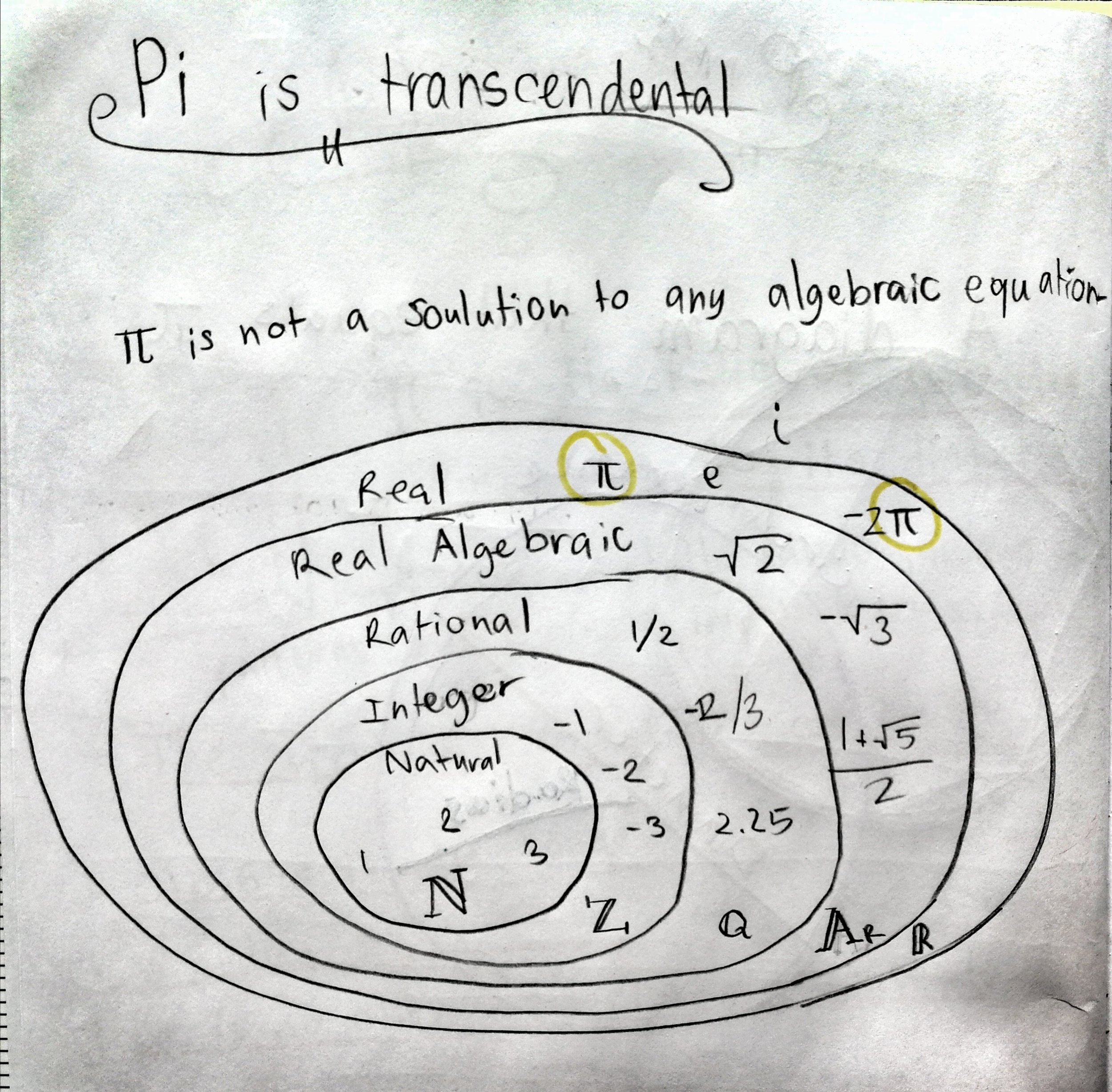
Here's the bit of Evie's book where she explains a bit about transcendental numbers.

Evie's book shows the relationships between the sets of natural numbers (N), integers (Z), rationals (Q), algebraic numbers (A), and real numbers (R). Transcendental numbers are real, but not algebraic. (Some definitions also let them be complex.)

Evie's book shows the relationships between the sets of natural numbers (N), integers (Z), rationals (Q), algebraic numbers (A), and real numbers (R). Transcendental numbers are real, but not algebraic. (Some definitions also let them be complex.)

I was interested in this, because while I 'knew' that pi is transcendental, I couldn't really articulate what that really meant, and why (say) √2, which is also irrational, is not also transcendental. Succinctly, transcendental means 'non-algebraic' (equivalent to being non-constructible). Since √2 is obviously the solution to \(x^2 - 2 = 0\), it is algebraic and therefore not transcendental. 

Weirdly, although hardly any numbers are known to be transcendental, almost all real numbers are. Isn't maths awesome?

Have a transcendental pi day!


The xkcd comic is by Randall Munroe and licensed CC-BY-NC.

Jounce, Crackle and Pop

jerk_shirt.png

I saw this T-shirt recently, and didn't get it. (The joke or the T-shirt.)

It turns out that the third derivative of displacement \(x\) with respect to time \(t\) — that is, the derivative of acceleration \(\mathbf{a}\) — is called 'jerk' (or sometimes, boringly, jolt, surge, or lurch) and is measured in units of m/s³. 

So far, so hilarious, but is it useful? It turns out that it is. Since the force \(\mathbf{F}\) on a mass \(m\) is given by \(\mathbf{F} = m\mathbf{a}\), you can think of jerk as being equivalent to a change in force. The lurch you feel at the onset of a car's acceleration — that's jerk. The designers of transport systems and rollercoasters manage it daily.

$$ \mathrm{jerk,}\ \mathbf{j} = \frac{\mathrm{d}^3 x}{\mathrm{d}t^3}$$

Here's a visualization of velocity (green line) of a Tesla Model S driving in a parking lot. The coloured stripes show the acceleration (upper plot) and the jerk (lower plot). Notice that the peaks in jerk correspond to changes in acceleration.

jerk_velocity_acceleration.png
jerk_velocity_jerk.png

The snap you feel at the start of the lurch? That's jounce  — the fourth derivative of displacement and the derivative of jerk. Eager et al (2016) wrote up a nice analysis of these quantities for the examples of a trampolinist and roller coaster passenger. Jounce is sometimes called snap... and the next two derivatives are called crackle and pop. 

What about momentum?

If the momentum \(\mathrm{p}\) of a mass \(m\) moving at a velocity \(v\) is \(m\mathbf{v}\) and \(\mathbf{F} = m\mathbf{a}\), what is mass times jerk? According to the physicist Philip Gibbs, who investigated the matter in 1996, it's called yank:

Momentum equals mass times velocity.
Force equals mass times acceleration.
Yank equals mass times jerk.
Tug equals mass times snap.
Snatch equals mass times crackle.
Shake equals mass times pop.

There are jokes in there, help yourself.

What about integrating?

Clearly the integral of jerk is acceleration, and that of acceleration is velocity, the integral of which is displacement. But what is the integral of displacement with respect to time? It's called absement, and it's a pretty peculiar quantity to think about. In the same way that an object with linearly increasing displacement has constant velocity and zero acceleration, an object with linearly increasing absement has constant displacement and zero velocity. (Constant absement at zero displacement gives rise to the name 'absement': an absence of displacement.)

Integrating displacement over time might be useful: the area under the displacement curve for a throttle lever could conceivably be proportional to fuel consumption for example. So absement seems to be a potentially useful quantity, measured in metre-seconds.

Integrate absement and you get absity (a play on 'velocity'). Keep going and you get abseleration, abserk, and absounce. Are these useful quantities? I don't think so. A quick look at them all — for the same Tesla S dataset I used before — shows that the loss of detail from multiple cumulative summations makes for rather uninformative transformations: 

jerk_jounce_etc.png

You can reproduce the figures in this article with the Jupyter Notebook Jerk_jounce_etc.ipynb. Or you can launch a Binder right here in your browser and play with it there, without installing a thing!


References

David Eager et al (2016). Beyond velocity and acceleration: jerk, snap and higher derivatives. Eur. J. Phys. 37 065008. DOI: 10.1088/0143-0807/37/6/065008

Amarashiki (2012). Derivatives of position. The Spectrum of Riemannium blog, retrieved on 4 Mar 2018.

The dataset is from Jerry Jongerius's blog post, The Tesla (Elon Musk) and
New York Times (John Broder) Feud
. I have no interest in the 'feud', I just wanted a dataset.

The T-shirt is from Chummy Tees; the image is their copyright and used here under Fair Use terms.

The vintage Snap, Crackle and Pop logo is copyright of Kellogg's and used here under Fair Use terms.

Finding Big Bertha with a hot wire

mcnaughton-canada-war-museum.jpg

Sunday will be the 131st birthday of General Andrew McNaughton, a Canadian electrical engineer who served in the Canadian Expeditionary Force in the First World War. He was eventually appointed commander of the Canadian Corps Heavy Artillery and went on to serve in the Second World War as well.

So what is a professional soldier doing on a blog about geoscience? Well, McNaughton was part of the revolution of applied acoustics and geophysics that emerged right before and after the First World War.

Along with eminent British physicist Lawrence Bragg, engineer William Sansome Tucker, and physicist Charles Galton Darwin (the other Charles Darwin's grandson), among others, McNaughton applied physics to the big problem of finding the big noisy things that were trying to blow everyone up. They were involved in an arms race of their own — German surveyor Ludger Mintrop was trying to achieve the same goal from the other side of the trenches.

Big_Bertha.jpg

After gaining experience as a gunner, McNaughton became one of a handful of scientists and engineers involved in counter-battery operations. Using novel ranging techniques, these scientists gave the allied forces a substantial advantage over the enemy. Counter-battery fire became an weapon at pivotal battles like Vimy Ridge, and certainly helped expedite the end of the war.

If all this sounds like a marginal way to win a battle, stop think for a second about these artillery. The German howitzer, known as 'Big Bertha' (left), could toss an 820 kg (1800 lb) shell about 12.5 km (7.8 miles). In other words, it was incredibly annoying.


Combining technologies

Localization accuracy on the order of 5–10 m on the large majority of gun positions was eventually achieved by the coordinated use of several technologies, including espionage, cartography, aerial reconnaissance photography, and the new counter-measures of flash spotting and sound ranging.

Flash spotting was more or less just what it sounds like: teams of spotters recording the azimuth of artillery flashes, then triangulating artillery positions from multiple observations. The only real trick was in reporting the timing of flashes to help establish that the flashes came from the same gun.

Sound ranging, on the other hand, is a tad more complicated. It seems that Lawrence Bragg was the first to realize that the low frequency sound of artillery fire — which he said lifted him off the privy seat in the outhouse at his lodgings — might be a useful signal. However, microphones were not up to the task of detecting such low frequencies. Furthermore, the signal was masked by the (audible) sonic boom of the shell, as well as the shockwaves of passing shells.

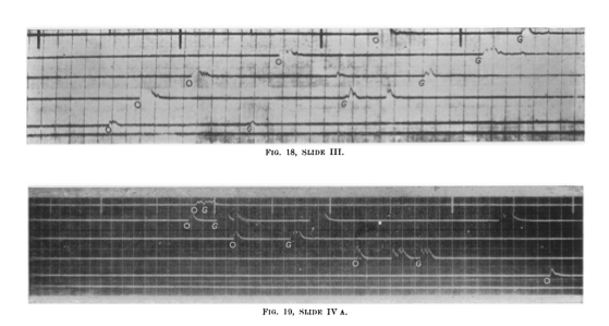
Elsewhere in Belgium, William Tucker had another revelation. Lying inside a shack with holes in its walls, he realized that the 20 Hz pressure wave from the gun created tiny puffs of air through the holes. So he looked for a way to detect this pulse, and came up with a heated platinum wire in a rum jar. The filament's resistance dropped when cooled by the wavefront's arrival through an aperture. The wire was unaffected by the high-frequency shell wave. Later, moving-coil 'microphones' (geophones, essentially) were also used, as well as calibration for wind and temperature. The receivers were coupled with a 5-channel string galvanometer, invented by French engineers, to record traces onto 35-mm film bearing timing marks:

sound-ranging-traces.png

McNaughton continued to develop these technologies through the war, and by the end was successfully locating the large majority of enemy artillery locations, and was even able to specify the calibre of the guns and their probable intended targets. Erster Generalquartiermeister Erich Ludendorff commented at one point in the war: 

According to a captured English document the English have a well- developed system of sound-ranging which in theory corresponds to our own. Precautions are accordingly to be taken to camouflage the sound: e.g. registration when the wind is contrary, and when there is considerable artillery activity, many batteries firing at the same time, simultaneous firing from false positions, etc.

An acoustic arsenal

Denge_acoustic_mirrors_March-2005_Paul-Russon.jpg

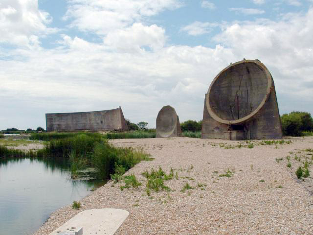
The hot-wire artillery detector was not Tucker's only acoustic innovation. He also pioneered the use of acoustic mirrors for aircraft detection. Several of these were built around the UK's east coast, starting around 1915 — the three shown here are at Denge in Kent. They were rendered obselete by the invention of radar around the beginning of World War Two.

Acoustic and seismic devices are still used today in military and security applications, though they are rarely mentioned in applied geophysics textbooks. If you know about any interesting contemporary uses, tell us about it in the comments.


According to Crown Copyright terms, the image of McNaughton is out of copyright. The acoustic mirror image is by Paul Russon, licensed CC-BY-SA. The uncredited/unlicensed galvanometer trace is from the excellent Stop, hey, what's that sound article on the geographical imaginations blog; I assume it is out of copyright. The howitzer image is out of copyright.

This post on Target acquisition and counter battery is very informative and has lots of technical details, though most of it pertains to later technology. The Boom! Sounding out the enemy article on ScienceNews for Students is also very nice, with lots of images. 

Unsolved problems in applied geoscience

I like unsolved problems. I first wrote about them way back in late 2010 — Unsolved problems was the eleventh post on this blog. I touched on the theme again in 2013, before and after the first 'unsession' at the GeoConvention, which itself was dedicated to finding the most pressing questions in exploration geoscience. As we turn towards the unsession at AAPG in Salt Lake City in May, I find myself thinking again about unsolved problems. Specifically, what are they? How can we find them? And what can we do to make them easier to solve?

It turns out lots of people have asked these questions before.

unsolved_problems.png

I've compiled a list of various attempts by geoscientists to list he big questions in the field. The only one I was previous aware of was Milo Backus's challenges in applied seismic geophysics, laid out in his president's column in GEOPHYSICS in 1980 and highlighted later by Larry Lines as part of the SEG's 75th anniversary. Here are some notable attempts:

  • John William Dawson, 1883 — Nova Scotia's most famous geologist listed unsolved problems in geology in his presidential address to the American Association for the Advancement of Science. They included the Cambrian Explosion, and the origin of the Antarctic icecap. 
  • Leason Heberling Adams, 1947 — One of the first experimental rock physicists, Adams made the first list I can find in geophysics, which was less than 30 years old at the time. He included the origin of the geomagnetic field, and the temperature of the earth's interior.
  • Milo Backus, 1980 — The list included direct hydrocarbon detection, seismic imaging, attenuation, and anisotropy.  
  • Mary Lou Zoback, 2000 — As her presidential address to the GSA, Zoback kept things quite high-level, asking questions about finding signal indynamic systems, defining mass flux and energy balance, identifying feedback loops, and communicating uncertainty and risk. This last one pops up in almost every list since.
  • Calgary's geoscience community, 2013 — The 2013 unsession unearthed a list of questions from about 50 geoscientists. They included: open data, improving seismic resolution, dealing with error and uncertainty, and global water management.
  • Daniel Garcia-Castellanos, 2014 — The Retos Terrícolas blog listed 49 problems in 7 categories, ranging from the early solar system to the earth's interior, plate tectonics, oceans, and climate. The list is still maintained by Daniel and pops up occasionally on other blogs and on Wikipedia.

The list continues — you can see them all in this presentation I made for a talk (online) at the Bureau of Economic Geology last week (thank you to Sergey Fomel for hosting me!). During the talk, I took the opportunity to ask those present what their unsolved problems are, especially the ones in their own fields. Here are a few of what we got (the rest are in the preso):

1-what-are-the-biggest-unsolved-problems-in-your-field-1.jpg

What are your unsolved problems in applied geoscience? Share them in the comments!


If you have about 50 minutes to spare, you can watch the talk here, courtesy of BEG's streaming service.

Click here to watch the talk >>>

What is scientific computing?

I started my career in sequence stratigraphy, so I know a futile discussion about semantics when I see one. But humour me for a second.

As you may know, we offer a multi-day course on 'geocomputing'. Somebody just asked me: what is this mysterious, made-up-sounding discipline? Swiftly followed by: can you really teach people how to do computational geoscience in a few days? And then: can YOU really teach people anything??

Good questions

You can come at the same kind of question from different angles. For example, sometimes professional programmers get jumpy about programming courses and the whole "learn to code" movement. I think the objection is that programming is a profession, like other kinds of engineering, and no-one would dream of offering a 3-day course on, say, dentistry for beginners.

These concerns are valid, sort of.

  1. No, you can't learn to be a computational scientist in 3 days. But you can make a start. A really good one at that.
  2. And no, we're not programmers. But we're scientists who get things done with code. And we're here to help.
  3. And definitely no, we're not trying to teach people to be software engineers. We want to see more computational geoscientists, which is a different thing entirely.

So what's geocomputing then?

Words seem inadequate for nuanced discussion. Let's instead use the language of ternary diagrams. Here's how I think 'scientific computing' stacks up against 'computer science' and 'software engineering'...

If you think these are confusing, just be glad I didn't go for tetrahedrons.

These are silly, of course. We could argue about them for hours I'm sure. Where would IT fit? ("It's all about the business" or something like that.) Where does Agile fit? (I've caricatured our journey, or tried to.) Where do you fit? 

The Surmont Supermerge

In my recent Abstract horror post, I mentioned an interesting paper in passing, Durkin et al. (2017):


Paul R. Durkin, Ron L. Boyd, Stephen M. Hubbard, Albert W. Shultz, Michael D. Blum (2017). Three-Dimensional Reconstruction of Meander-Belt Evolution, Cretaceous Mcmurray Formation, Alberta Foreland Basin, Canada. Journal of Sedimentary Research 87 (10), p 1075–1099. doi: 10.2110/jsr.2017.59


I wanted to write about it, or rather about its dataset, because I spent about 3 years of my life working on the USD 75 million seismic volume featured in the paper. Not just on interpreting it, but also on acquiring and processing the data.

Let's start by feasting our eyes on a horizon slice, plus interpretation, of the Surmont 'Supermerge' 3D seismic volume:

Figure 1 from Durkin et al (2017), showing a stratal slice from 10 ms below the top of the McMurray Formation (left), and its interpretation (right). © 2017, SEPM (Society for Sedimentary Geology) and licensed CC-BY.

Figure 1 from Durkin et al (2017), showing a stratal slice from 10 ms below the top of the McMurray Formation (left), and its interpretation (right). © 2017, SEPM (Society for Sedimentary Geology) and licensed CC-BY.

A decade ago, I was 'geophysics advisor' on Surmont, which is jointly operated by ConocoPhillips Canada, where I worked, and Total E&P Canada. My line manager was a Total employee; his managers were ex-Gulf Canada. It was a fantastic, high-functioning team, and working on this project had a profound effect on me as a geoscientist. 

The Surmont bitumen field

The dataset covers most of the Surmont lease, in the giant Athabasca Oil Sands play of northern Alberta, Canada. The Surmont field alone contains something like 25 billions barrels of bitumen in place. It's ridiculously massive — you'd be delighted to find 300 million bbl offshore. Given that it's expensive and carbon-intensive to produce bitumen with today's methods — steam-assisted gravity drainage (SAGD, "sag-dee") in Surmont's case — it's understandable that there's a great deal of debate about producing the oil sands. One factoid: you have to burn about 1 Mscf or 30 m³ of natural gas, costing about USD 10–15, to make enough steam to produce 1 bbl of bitumen.

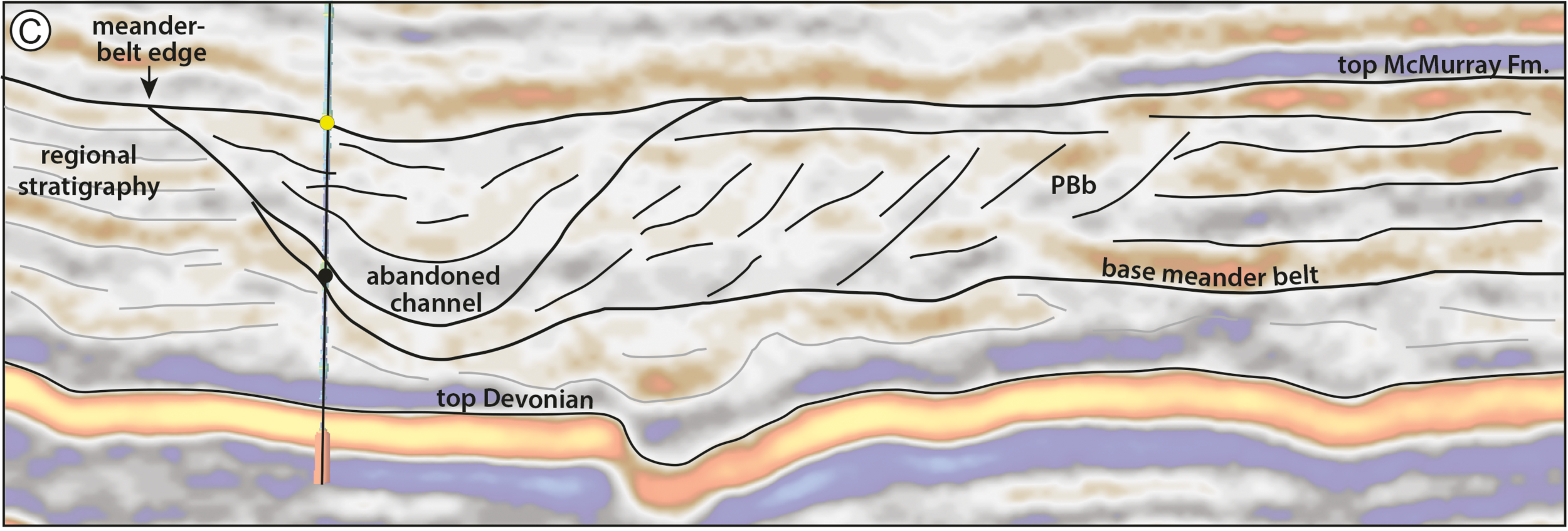
Detail from Figure 12 from Durkin et al (2017), showing a seismic section through the McMurray Formation. Most of the abandoned channels are filled with mudstone (really a siltstone). The dipping heterolithic strata of the point bars, so obvious in …

Detail from Figure 12 from Durkin et al (2017), showing a seismic section through the McMurray Formation. Most of the abandoned channels are filled with mudstone (really a siltstone). The dipping heterolithic strata of the point bars, so obvious in horizon slices, are quite subtle in section. © 2017, SEPM (Society for Sedimentary Geology) and licensed CC-BY.

The field is a geoscience wonderland. Apart from the 600 km² of beautiful 3D seismic, there are now about 1500 wells, most of which are on the 3D. In places there are more than 20 wells per section (1 sq mile, 2.6 km², 640 acres). Most of the wells have a full suite of logs, including FMI in 2/3 wells and shear sonic as well in many cases, and about 550 wells now have core through the entire reservoir interval — about 65–75 m across most of Surmont. Let that sink in for a minute.

What's so awesome about the seismic?

OK, I'm a bit biased, because I planned the acquisition of several pieces of this survey. There are some challenges to collecting great data at Surmont. The reservoir is only about 500 m below the surface. Much of the pay sand can barely be called 'rock' because it's unconsolidated sand, and the reservoir 'fluid' is a quasi-solid with a viscosity of 1 million cP. The surface has some decent topography, and the near surface is glacial till, with plenty of boulders and gravel-filled channels. There are surface lakes and the area is covered in dense forest. In short, it's a geophysical challenge.

Nonetheless, we did collect great data; here's how:

  • General information
    • The ca. 600 km² Supermerge consists of a dozen 3Ds recorded over about a decade starting in 2001.
    • The northern 60% or so of the dataset was recombined from field records into a single 3D volume, with pre- and post-stack time imaging.
    • The merge was performed by CGG Veritas, cost nearly $2 million, and took about 18 months.
  • Geometry
    • Most of the surveys had a 20 m shot and receiver spacing, giving the volume a 10 m by 10 m natural bin size
    • The original survey had parallel and coincident shot and receiver lines (Megabin); later surveys were orthogonal.
    • We varied the line spacing between 80 m and 160 m to get trace density we needed in different areas.
  • Sources
    • Some surveys used 125 g dynamite at a depth of 6 m; others the IVI EnviroVibe sweeping 8–230 Hz.
    • We used an airgun on some of the lakes, but the data was terrible so we stopped doing it.
  • Receivers
    • Most of the surveys were recorded into single-point 3C digital MEMS receivers planted on the surface.
  • Bandwidth
    • Most of the datasets have data from about 8–10 Hz to about 180–200 Hz (and have a 1 ms sample interval).

The planning of these surveys was quite a process. Because access in the muskeg is limited to 'freeze up' (late December until March), and often curtailed by wildlife concerns (moose and elk rutting), only about 6 weeks of shooting are possible each year. This means you have to plan ahead, then mobilize a fairly large crew with as many channels as possible. After acquisition, each volume spent about 6 months in processing — mostly at Veritas and then CGG Veritas, who did fantastic work on these datasets.

Kudos to ConocoPhillips and Total for letting people work on this dataset. And kudos to Paul Durkin for this fine piece of work, and for making it open access. I'm excited to see it in the open. I hope we see more papers based on Surmont, because it may be the world's finest subsurface dataset. I hope it is released some day, it would have huge impact.


References & bibliography

Paul R. Durkin, Ron L. Boyd, Stephen M. Hubbard, Albert W. Shultz, Michael D. Blum (2017). Three-Dimensional Reconstruction of Meander-Belt Evolution, Cretaceous Mcmurray Formation, Alberta Foreland Basin, Canada. Journal of Sedimentary Research 87 (10), p 1075–1099. doi: 10.2110/jsr.2017.59 (not live yet).

Hall, M (2007). Cost-effective, fit-for-purpose, lease-wide 3D seismic at Surmont. SEG Development and Production Forum, Edmonton, Canada, July 2007.

Hall, M (2009). Lithofacies prediction from seismic, one step at a time: An example from the McMurray Formation bitumen reservoir at Surmont. Canadian Society of Exploration Geophysicists National Convention, Calgary, Canada, May 2009. Oral paper.

Zhu, X, S Shaw, B Roy, M Hall, M Gurch, D Whitmore and P Anno (2008). Near-surface complexity masquerades as anisotropy. SEG Annual Convention, Las Vegas, USA, November 2008. Oral paper. doi: 10.1190/1.3063976.

Surmont SAGD Performance Review (2016), by ConocoPhillips and Total geoscientists and engineers. Submitted to AER, 258 pp. Available online [PDF] — and well worth looking at.

Trad, D, M Hall, and M Cotra (2008). Reshooting a survey by 5D interpolation. Canadian Society of Exploration Geophysicists National Convention, Calgary, Canada, May 2006. Oral paper.