Cross plots: a non-answer

On Monday I asked whether we should make crossplots according to statistical rules or natural rules. There was some fun discussion, and some awesome computation from Henry Herrera, and a couple of gems:

Physics likes math, but math doesn't care about physics — @jeffersonite

But... when I consider the intercept point I cannot possibly imagine a rock that has high porosity and zero impedance — Matteo Niccoli, aka @My_Carta

I tried asking on Stack Overflow once, but didn’t really get to the bottom of it, or perhaps I just wasn't convinced. The consensus seems to be that the statistical answer is to put porosity on y-axis, because that way you minimize the prediction error on porosity. But I feel—and this is just my flaky intuition talking—like this fails to represent nature (whatever that means) and so maybe that error reduction is spurious somehow.

Reversing the plot to what I think of as the natural, causation-respecting plot may not be that unreasonable. It's effectively the same as reducing the error on what was x (that is, impedance), instead of y. Since impedance is our measured data, we could say this regression respects the measured data more than the statistical, non-causation-respecting plot.
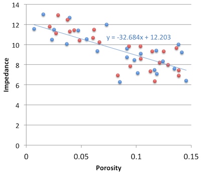
So must we choose? Minimize the error on the prediction, or minimize the error on the predictor. Let's see. In the plot on the right, I used the two methods to predict porosity at the red points from the blue. That is, I did the regression on the blue points; the red points are my blind data (new wells, perhaps). Surprisingly, the statistical method gives an RMS error of 0.034, the natural method 0.023. So my intuition is vindicated! 

Unfortunately if I reverse the datasets and instead model the red points, then predict the blue, the effect is also reversed: the statistical method does better with 0.029 instead of 0.034. So my intuition is wounded once more, and limps off for an early bath.

Irreducible error?

Here's what I think: there's an irreducible error of prediction. We can beg, borrow or steal error from one variable, but then it goes on the other. It's reminiscent of Heisenberg's uncertainty principle, but in this case, we can't have arbitrarily precise forecasts from imperfectly correlated data. So what can we do? Pick a method, justify it to yourself, test your assumptions, and then be consistent. And report your errors at every step. 

I'm reminded of the adage 'Correlation does not equal causation.' Indeed. And, to borrow @jeffersonite's phrase, it seems correlation also does not care about causation.

Reliable predictions of unlikely geology

A puzzle

Imagine you are working in a newly-accessible and under-explored area of an otherwise mature basin. Statistics show that on average 10% of structures are filled with gas; the rest are dry. Fortunately, you have some seismic analysis technology that allows you to predict the presence of gas with 80% reliability. In other words, four out of five gas-filled structures test positive with the technique, and when it is applied to water-filled structures, it gives a negative result four times out of five.

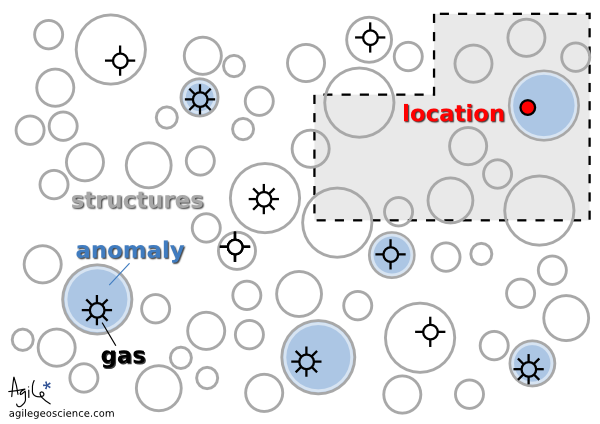
It is thought that 10% of the structures in this play are gas-filled. Your seismic attribute test is thought to be 80% reliable, because four out of five times it has indicated gas correctly. You acquire the undrilled acreage shown by the grey polygon.

You acquire some undrilled acreage—the grey polygon— then delineate some structures and perform the analysis. One of the structures tests positive. If this is the only information you have, what is the probability that it is gas-filled?

This is a classic problem of embracing Bayesian likelihood and ignoring your built-in 'representativeness heuristic' (Kahneman et al, 1982, Judgment Under Uncertainty: Heuristics and Biases, Cambridge University Press). Bayesian probability combination does not come very naturally to most people but, once understood, can at least help you see the way to approach similar problems in the future. The way the problem is framed here, it is identical to the original formulation of Kahneman et al, the Taxicab Problem. This takes place in a town with 90 yellow cabs and 10 blue ones. A taxi is involved in a hit-and-run, witnessed by a passer-by. Eye witness reliability is shown to be 80%, so if the witness says the taxi was blue, what is the probability that the cab was indeed blue? Most people go with 80%, but in fact the witness is probably wrong. To see why, let's go back to the exploration problem and look at 100 test cases.

Break it down

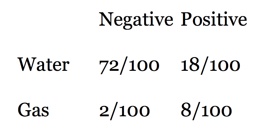
Looking at the rows in this table of outcomes, we see that there are 90 water cases and 10 gas cases. Eighty percent of the water cases test negative, and 80% of the gas cases test positive. The table shows that when we get a positive test, the probability that the test is true is not 0.80, but much less: 8/(8+18) = 0.31. In other words, a test that is mostly reliable is probably wrong when applied to an event that doesn't happen very often (a structure being gas charged). It's still good news for us, though, because a probability of discovery of 0.31 is much better than the 0.10 that we started with.

Here is Bayes' Theorem for calculating the probability P of event A (say, a gas discovery) given event B (say, a positive test in our seismic analysis):

So we can express our problem in these terms:

Are you sure about that?

This result is so counter-intuitive, for me at least, that I can't resist illustrating it with another well-known example that takes it to extremes. Imagine you test positive for a very rare disease, seismitis. The test is 99% reliable. But the disease affects only 1 person in 10 000. What is the probability that you do indeed have seismitis?

Notice that the unreliability (1%) of the test is much greater than the rate of occurrence of the disease (0.01%). This is a red flag. It's not hard to see that there will be many false positives: only 1 person in 10 000 are ill, and that person tests positive 99% of the time (almost always). The problem is that 1% of the 9 999 healthy people, 100 people, will test positive too. So for every 10 000 people tested, 101 test positive even though only 1 is ill. So the probability of being ill, given a positive test, is only about 1/101!

Lessons learned

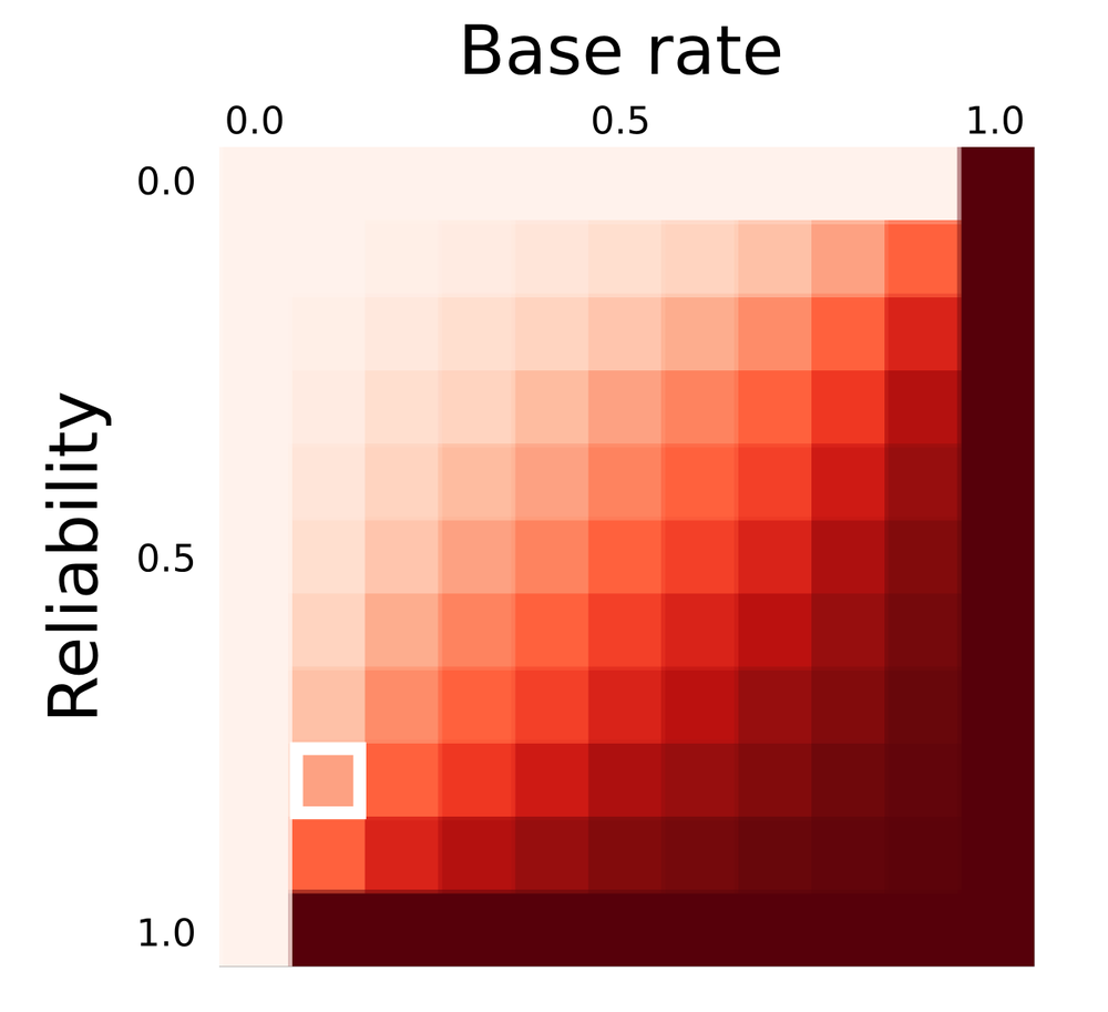
Predictive power (in Bayesian jargon, the posterior probability) as a function of test reliability and the base rate of occurrence (also called the prior probability of the event of phenomenon in question). The position of the scenario in the exploration problem is shown by the white square.

Thanks to UBC Bioinformatics for the heatmap software, heatmap.notlong.com.


Next time you confidently predict something with a seismic attribute, stop to think not only about the reliability of the test you have made, but the rate of occurrence of the thing you're trying to predict. The heatmap shows how prediction power depends on both test reliability and the occurrence rate of the event. You may be doing worse (or better!) than you think.

Fortunately, in most real cases, there is a simple mitigation: use other, independent, methods of prediction. Mutually uncorrelated seismic attributes, well data, engineering test results, if applied diligently, can improve the odds of a correct prediction. But computing the posterior probability of event A given independent observations B, C, D, E, and F, is beyond the scope of this article (not to mention this author!).

This post is a version of part of my article The rational geoscientist, The Leading Edge, May 2010

How to cheat

Yesterday I posted the rock physics cheatsheet, which is a condensed version of useful seismic reservoir characterization and rock mechanics concepts. It's cheat as in simplify, not cheat as in swindle. 

As Matt discussed on Friday, heuristics can be shortcuts to hone your intuition. Our minds search to use rules of thumb to visualise the invisible and to solve sticky problems. That's where the cheat sheet comes in. You might not find rock physics that intuitive, but let's take a look at the table to see how it reveals some deeper patterns.

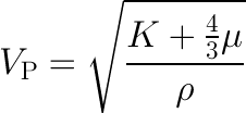
The table of elastic parameters is setup based on the fundamental notion that, if you have any two elastic properties previously defined, you can compute all the others. This is a consequence of one of the oldest laws in classical mechanics: Newton's second law, F=ma. In particular one thing I find profound about seismic velocity is that it is wholly determined by a ratio of competing tensional (elastic) forces to inertial (density) forces. To me, it is not immediately obvious that speed, with units of m/s, results from the ratio of pressure to density. 

This simple little equation has had a profound impact on the utility of seismology to the oil and gas industry. It links extrinsic dynamic properties (VP) to intrinsic rock properties (K, μ, ρ). The goal of course, is not just to investigate elastic properties for the sake of it, but to link elastic properties to reservoir and petrophysical properties. This is traditionally done using a rock physics template. The one I find easiest to understand is the VP/VS vs P-impedance template, an example of which is shown on the cheatsheet. You will see others in use, for instance Bill Goodway has pioneered the λρ vs μρ (LMR) template.

In an upcoming post we'll look to deepen the connection between Newtonian mechanics and reservoir characterization. 

Confirmation

The first principle is that you must not fool yourself — and you are the easiest person to fool. So you have to be very careful about that. After you've not fooled yourself, it's easy not to fool other scientists.
Richard Feynman, 1974

Suppose that I have done a seismic inversion and have a new seismic attribute volume that predicts Poisson's ratio (a rock property that can help predict fluid type). According to my well calibration and my forward modelling, low Poisson's ratio means Gas. This is my hypothesis; I need to test it.

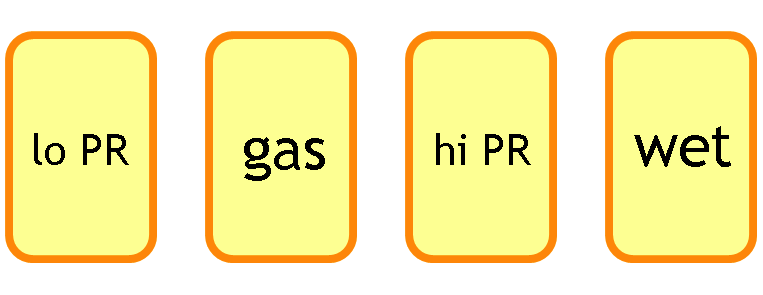
So here's a game: I have some new wells, represented by double-sided cards. Which cards do I need to turn over to prove the hypothesis that all the cards with Low PR on one side have Gas on the other? Take a moment to look at the four cards and decide which you will flip:

In the course of evolution, our brains have developed heuristics, rules of thumb, for dealing with problems like this one. Our intuition is made of heuristics: we're wary of the outsider with the thick accent; we balk at a garden hose in the grass that could have been a snake. We are programmed to see faces in the topography of Mars (left). The rules are useful to us in urgent matters of survival, letting us take the least risky course of urgent action. But I think they're limiting and misleading when rational decisions are required.

That's why most people, even educated people, get this problem wrong. As scientists we should be especially wary of this, but the fact is that we all tend to seek information that confirms our hypotheses, rather than trying to disprove them. In the problem above, the cards to flip are the Low PR card (of course, it had better have Gas on the other side), and the Water card, because it had better not say Low PR. Most people select the Gas card, but it is not required because its reverse cannot prove our disprove our hypothesis: we don't care if High PR also means Gas sometimes (or even all the time).

Think of a hypothesis you have about the data you are working on right now. Can you think of a test that might disprove it? Would you get funding for a test like this? 

This post is a version of part of my article The rational geoscientist, The Leading Edge, May 2010. I recently read this post on the OpenScience Project blog, and it got me thinking about this again. The image of Mars was created by NASA and the JPL, and is in the public domain.