Which brittleness index?

A few weeks ago I looked at the concept — or concepts — of brittleness. There turned out to be lots of ways of looking at it. We decided to call it a rock behaviour rather than a property. And we determined to look more closely at some different ways to define it. Here they are...

Some brittleness indices

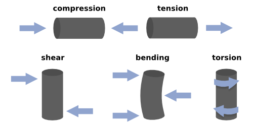
There are lots of 'definitions' of brittleness in the literature. Several of them capture the relationship between compressive and tensile strength, σ_C and σ_T respectively. This is potentially useful, because we measure uniaxial compressive strength in the standard triaxial rig tests that have become routine in shale studies... but we don't usually find the tensile strength, because it's much harder to measure. This is unfortunate, because hydraulic fracturing is initially a tensile failure (though reactivation and other failure modes do occur — see Williams-Stroud et al. 2012).

Altindag (2003) gave the following three examples of different brittleness indices. In turn, they are the strength ratio, a sort of relative strength contrast, and the mean strength (his favourite):

This is just the start, once you start digging, you'll find lots of others. Like Hucka & Das's (1974) round-up I wrote about last time, one thing they have in common is that they capture some characteristic of rock failure. That is, they do not rely on implicit rock properties.

Another point to note. Bažant & Kazemi (1990) gave a way to de-scale empirical brittleness measures to account for sample size — not surprisingly, this sort of 'real world adjustment' starts to make things quite complicated. Not so linear after all.

What not to do

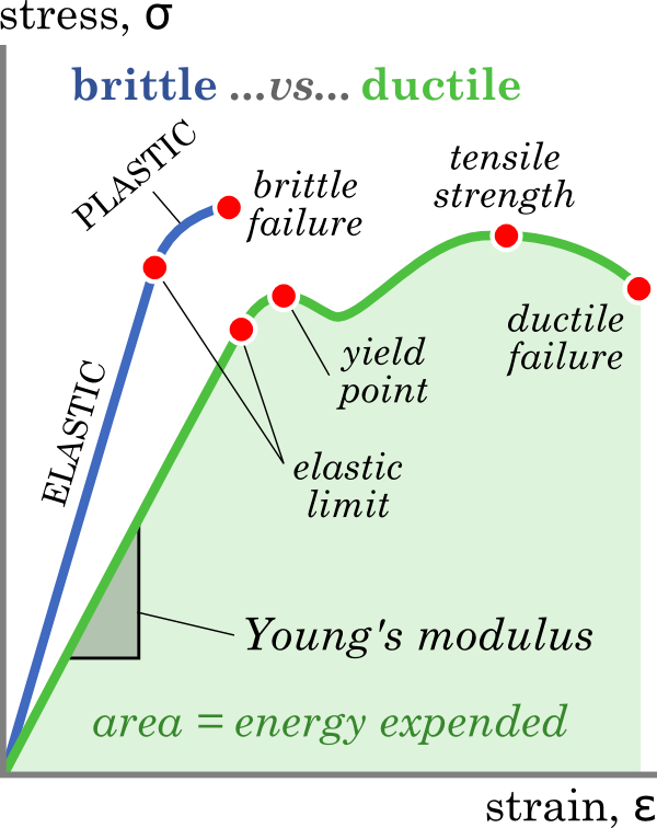
The prevailing view among many interpreters is that brittleness is proportional to Young's modulus and/or Poisson's ratio, and/or a linear combination of these. We've reported a couple of times on what Lev Vernik (Marathon) thinks of the prevailing view: we need to question our assumptions about isotropy and linear strain, and computing shale brittleness from elastic properties is not physically meaningful. For one thing, you'll note that elastic moduli don't have anything to do with rock failure.

The Young–Poisson brittleness myth started with Rickman et al. 2008, SPE 115258, who presented a rather ugly representation of a linear relationship (I gather this is how petrophysicists like to write equations). You can see the tightness of the relationship for yourself in the data.

If I understand  the notation, this is the same as writing B = 7.14E – 200ν + 72.9, where E is (static) Young's modulus and ν is (static) Poisson's ratio. It's an empirical relationship, based on the data shown, and is perhaps useful in the Barnett (or wherever the data are from, we aren't told). But, as with any kind of inversion, the onus is on you to check the quality of the calibration in your rocks. 

What's left?

Here's Altindag (2003) again:

Brittleness, defined differently from author to author, is an important mechanical property of rocks, but there is no universally accepted brittleness concept or measurement method...

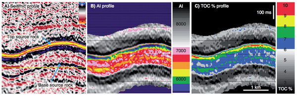
This leaves us free to worry less about brittleness, whatever it is, and focus on things we really care about, like organic matter content or frackability (not unrelated). The thing is to collect good data, examine it carefully with proper tools (Spotfire, Tableau, R, Python...) and find relationships you can use, and prove, in your rocks.

References

Altindag, R (2003). Correlation of specific energy with rock brittleness concepts on rock cutting. The Journal of The South African Institute of Mining and Metallurgy. April 2003, p 163ff. Available online.

Hucka V, B Das (1974). Brittleness determination of rocks by different methods. Int J Rock Mech Min Sci Geomech Abstr 10 (11), 389–92. DOI:10.1016/0148-9062(74)91109-7.

Rickman, R, M Mullen, E Petre, B Grieser, and D Kundert (2008). A practical use of shale petrophysics for stimulation design optimization: all shale plays are not clones of the Barnett Shale. SPE 115258, DOI: 10.2118/115258-MS.

Williams-Stroud, S, W Barker, and K Smith (2012). Induced hydraulic fractures or reactivated natural fractures? Modeling the response of natural fracture networks to stimulation treatments. American Rock Mechanics Association 12–667. Available online.

What is brittleness?

Brittleness is an important rock characteristic, but impossible to define formally because there are so many different ways of looking at it. For this reason, Tiryaki (2006) suggests we call it a rock behaviour, not a rock property.

Indeed, we're not really interested in brittleness, per se, because it's not very practical information on its own. Mining engineers are concerned with a property called cuttability — and we can think of this as conceptually analogous to the property that interests lots of geologsts, geophysicists, and engineers in petroleum, geothermal, and hydrology: frackability. In materials science, the inverse property — the ability of a rock to resist fracture — is called fracture toughness. 

What is brittleness not?

• It's not the same as frackability, or other things you might be interested in.
• It's not a simple rock property like, say, density or velocity. Those properties are condition-dependent too, but we agree on how to measure them.
• It's not proportional to any elastic moduli, or a linear combination of Young's modulus and Poisson's ratio, despite what you might have heard.

So what is it then?

It depends a bit what you care about. How the rock deforms under stress? How much energy it takes to break it? What happens when it breaks? Hucka and Das (1974) rounded up lots of ways of looking at it. Here are a few:

• Brittle rocks undergo little to no permanent deformation before failure and, depending on the test conditions, may occur suddenly and catastrophically.
• Brittle rocks undergo little or no ductile deformation past the yield point (or elastic limit) of the rock. Note that some materials, including many rocks, have no well-defined yield point because they have non-linear elasticity.
• Brittle rocks absorb relatively little energy before fracturing. The energy absorbed is equal to the area under the stress-strain curve (see figure).
• Brittle rocks have a strong tendency to fracture under stress.
• Brittle rocks break with a high ratio of fine to coarse fragments.

All of this is only made more complicated by the fact that there are lots of kinds of stress: compression, tension, shear, torsion, bending, and impact... and all of these can operate in multiple dimensions, and on multiple time scales. Suddenly a uniaxial rig doesn't quite seem like enough kit.

It will take a few posts to really get at brittleness and frackability. In future posts we'll look at relevant rock properties and how to measure them, the difference between static and dynamic measurements, and the multitude of brittleness indices. Eventually, we'll get on to what all this means for seismic waves, and ask whether frackability is something we can reasonably estimate from seismic data.

Meanwhile, if you have observations or questions to share, hit us in the comments. 

References and further reading
Hucka V, B Das (1974). Brittleness determination of rocks by different methods. Int J Rock Mech Min Sci Geomech Abstr 10 (11), 389–92. DOI:10.1016/0148-9062(74)91109-7
Tiryaki (2006). Evaluation of the indirect measures of rock brittleness and fracture toughness in rock cutting. The Journal of The South African Institute of Mining and Metallurgy 106, June 2006. Available online.

Update on 2014-06-12 01:21 by Matt Hall

Don't miss the later post, Which brittleness index?

Submitting assumptions for meaningful answers

The best talk of the conference was Ran Bachrach's on seismics for unconventionals. He enthusiastically described the physics to his spectators with conviction and duty, and explained why they should care. Isotropic, VTI, and orthorhombic media anisotropy models are used not because they are right, but because they are simple. If the assumptions you bring to the problem are reasonable, the answers can be considered meaningful. If you haven't considered and tested your assumptions, you haven't subscribed to reason. In a sense, you haven't held up your end of the bargain, and there will never be agreement. This talk should be mandatory viewing for anyone working seismic for unconventionals. Advocacy for reason. Too bad it wasn't recorded.

I am both privileged and obliged to celebrate such nuggets of awesomeness. That's a big reason why I blog. And on the contrary, we should call out crappy talks when we see them to raise the bar. Indeed, to quote Zen Faulkes, "...we should start creating more of an expectation that scientific talks will be reviewed and critiqued. And names will be named."

The talk from HEF Petrophysical entitled, Towards modelling three-dimensional oil sands permeability distribution using borehole image logs, drew me in. I was curious enough to show up. But as the talk unfolded, my curiosity was left unsatisfied. A potentially interesting workflow of transforming high-resolution resistivity measurements into flow permeability was obfuscated with a pointless upscaling step. The meat of anything like this is in the transform itself, but it was missing. It's also the most trivial bit; just cross-plot one property with another and show people. So I am guessing they didn't have any permeability data. If that was the case, how can you stand up and talk about permeability? It was a sandwich without the filling. The essential thing that defines a piece of work is the creativity. The thing you add that wasn't there before. I was disappointed. Disappointed that it was accepted, and that no one else piped up. 

I will paraphrase a conversation I had with Ran at the coffee break: Some are not aware, some choose to ignore, and some forget that works of geoscience are problems of extreme complexity. In fact, the only way we can cope with complexity is to make certain assumptions that make our problem solvable. If all you do is say "here is my solution", you suck. But if instead you ask, "Have I convinced you that my assumptions are reasonable?", it entirely changes the conversation. It entirely changes the specialist's role. Only when you understand your assumptions can we talk about whether the results are reasonable. 

Have you ever felt conflicted on whether or not you should say something?

Brittleness and robovibes

Day 3 of the SEG Annual Meeting was just as rammed with geophysics as the previous two days. I missed this morning's technical program, however, as I've taken on the chairpersonship (if that's a word) of the SEG Online Committee. So I had fun today getting to grips with that business. Aside: if you have opinion's about SEG's online presence, please feel free to send them my way.

Here are my highlights from the rest of the day — both were footnotes in their respective talks:

Brittleness — Lev Vernick, Marathon

Evan and I have had a What is brittleness? post in our Drafts folder for almost two years. We're skeptical of the prevailing view that a shale's brittleness is (a) a tangible rock property and (b) a function of Young's modulus and Poisson's ratio, as proposed by Rickman et al. 2008, SPE 115258. To hear such an intellect as Lev declare the same today convinced me that we need to finish that post — stay tuned for that. Bottom line: computing shale brittleness from elastic properties is not physically meaningful. We need to find more appropriate measures of frackability, [Edit, May 2015; Vernik tells me the following bit is the opposite of what he said, apologies for my cloth ears...] which Lev pointed out is, generally speaking, inversely proportional to organic content. This poses a basic conflict for those exploiting shale plays. [End of public service announcement.]

Robovibes — Guus Berkhout, TU Delft

At least 75% of Berkhout's talk went by me today, mostly over my head. I stopped writing notes, which I only do when I'm defeated. But once he'd got his blended source stuff out of the way, he went rogue and asked the following questions:

1. Why do we combine all seismic frequencies into the device? Audio got over this years ago (right).
2. Why do we put all the frequencies at the same location? Viz 7.1 surround sound.
3. Why don't we try more crazy things in acquisition?

I've wondered the same thing myself — thinking more about the receiver side than the sources — after hearing about the brilliant sampling strategy the Square Kilometer Array is using at a PIMS Lunchbox Lecture once. But Berkhout didn't stop at just spreading a few low-frequency vibrators around the place. No, he wants robots. He wants an autonomous army of flying and/or floating narrow-band sources, each on its own grid, each with its own ghost matching, each with its own deblending code. This might be the cheapest million-channel acquisition system possible. Berkhout's aeronautical vibrator project starts in January. Seriously.

More posts from SEG 2012.

Speaker image is licensed CC-BY-SA by Tobias Rütten, Wikipedia user Metoc.

Source rocks from seismic

A couple of years ago, Statoil's head of exploration research, Ole Martinsen, told AAPG Explorer magazine about a new seismic analysis method. Not just another way to discriminate between sand and shale, or water and gas, this was a way to assess source rock potential. Very useful in under-explored basins, and Statoil developed it for that purpose, but only the very last sentence of the Explorer article hints at its real utility today: shale gas exploration.

Calling the method Source Rocks from Seismic, Martinsen was cagey about details, but the article made it clear that it's not rocket surgery: “We’re using technology that would normally be used, say, to predict sandstone and fluid content in sandstone,” said Marita Gading, a Statoil researcher. Last October Helge Løseth, along with Gading and others, published a complete account of the method (Løseth et al, 2011).

Because they are actively generating hydrocarbons, source rocks are usually overpressured. Geophysicists have used this fact to explore for overpressured zones and even shale before. For example, Mukerji et al (2002) outlined the rock physics basis for low velocities in overpressured zones. Applying the physics to shales, Liu et al (2007) suggested a three-step process for evaluating source rock potential in new basins: 1 Sequence stratigraphic interpretation; 2 Seismic velocity analysis to determine source rock thickness; 3 Source rock maturity prediction from seismic. Their method is also a little hazy, but the point is that people are looking for ways to get at source rock potential via seismic data. 

The Løseth et al article was exciting to see because it was the first explanation of the method that Statoil had offered. This was exciting enough that the publication was even covered by Greenwire, by Paul Voosen (@voooos on Twitter). It turns out to be fairly straightforward: acoustic impedance (AI) is inversely and non-linearly correlated with total organic carbon (TOC) in shales, though the relationship is rather noisy in the paper's examples (Kimmeridge Clay and Hekkingen Shale). This means that an AI inversion can be transformed to TOC, if the local relationship is known—local calibration is a must. This is similar to how companies estimate bitumen potential in the Athabasca oil sands (e.g. Dumitrescu 2009). 

Figure 6 from Løseth et al (2011). A Seismic section. B Acoustic impedance. C Inverted seismic section where source rock interval is converted to total organic carbon (TOC) percent. Seismically derived TOC percent values in source rock intervals can be imported to basin modeling software to evaluate hydrocarbon generation potential of a basin. Click for full size..The result is that thick rich source rocks tend to have strong negative amplitude at the top, at least in subsiding mud-rich basins like the North Sea and the Gulf of Mexico. Of course, amplitudes also depend on stratigraphy, tuning, and so on. The authors expect amplitudes to dim with offset, because of elastic and anisotropic effects, giving a Class 4 AVO response.

This is a nice piece of work and should find application worldwide. There's a twist though: if you're interested in trying it out yourself, you might be interested to know that it is patent-pending: 

WO/2011/026996
INVENTORS:  Løseth,  H;  Wensaas, L; Gading, M; Duffaut, K; Springer, HM
Method of assessing hydrocarbon source rock candidate
A method of assessing a hydrocarbon source rock candidate uses seismic data for a region of the Earth. The data are analysed to determine the presence, thickness and lateral extent of candidate source rock based on the knowledge of the seismic behaviour of hydrocarbon source rocks. An estimate is provided of the organic content of the candidate source rock from acoustic impedance. An estimate of the hydrocarbon generation potential of the candidate source rock is then provided from the thickness and lateral extent of the candidate source rock and from the estimate of the organic content.

References

Dumitrescu, C (2009). Case study of a heavy oil reservoir interpretation using Vp/Vs ratio and other seismic attributes. Proceedings of SEG Annual Meeting, Houston. Abstract is online. 

Liu, Z, M Chang, Y Zhang, Y Li, and H Shen (2007). Method of early prediction on source rocks in basins with low exploration activity. Earth Science Frontiers 14 (4), p 159–167. DOI 10.1016/S1872-5791(07)60031-1

Løseth, H, L Wensaas, M Gading, K Duffaut, and M Springer (2011). Can hydrocarbon source rocks be identified on seismic data? Geology 39 (12) p 1167–1170. First published online 21 October 2011. DOI 10.1130/​G32328.1

Mukerji, T, Dutta, M Prasad, J Dvorkin (2002). Seismic detection and estimation of overpressures. CSEG Recorder, September 2002. Part 1 and Part 2 (Dutta et al, same issue). 

The figure is reproduced from Løseth et al (2011) according to The Geological Society of America's fair use guidelines. Thank you GSA! The flaming Kimmeridge Clay photograph is public domain. 

Workshop? Talkshop

Day 4 of the SEG Annual Meeting. I attended the workshop entitled Geophysical data interpretation for unconventional reservoirs. It was really about the state of the art of seismic technologies for shale gas exploration and exploitation, but an emergent theme was the treatment of the earth as an engineering material, as opposed to an acoustic or elastic medium.

Harvey Goodman from Chevron started the workshop by asking the packed room, "are there any engineers in the room?" Hilariously, a single lonesome hand was raised. "Well," he said "this talk is for you." Perhaps this wasn't the venue for it; so much for spreading cross-disciplinary love and the geophysical technical vernacular. 

Mark Zoback from Stanford presented decades worth of laboratory measurements on the elastic/plastic properties of shales. Specifically the concentrations of illite and TOC on mechanical stiffness and creep. When it came to questions, he provided the most compentent and cogent responses of the day: every one was gold. Your go-to guy for shale geomechanics.

Marita Gading of Statoil presented some facinating technology called Source Rock from Seismic (we mentioned this on Monday)—a way to estimate total organic carbon from seismic for basin modeling and play evaluation. She listed the factors controling acoustic properties of shales as

1. organic content;
2. compaction or porosity;
3. lithotype and mineral composition;
4. seismic to microscale anisotropy.

She showed an empirically derived acoustic impedance transform coupled with more interpretive methods, and the results are compelling. It's not clear how well this might work in ancient shales onshore, but it has apparently worked for Statoil in younger, offshore basins.

Galen Treadgold from Global Geophysical gave a visually stunning presentation showing the value of expansive data sets in the Eagle Ford shale. He showed 1000 km² of 3D seismic that had been stitched together, highlighting the need to look at a regional picture. Patchwork data fails to give the same clarity of variation in mechanical stratigraphy.

The session shifted to the state of microseismic technology and 'getting beyond the dots'. Speakers from rival companies MicroSeismic, ESG Solutions, and Pinnacle described how microseismic waveforms are now being used to resolve moment tensors. These provide not only the location and magnitude but also the failure characteristic of every single event. While limited by uncertainty, they may be the way to get the industry beyond the prevailing bi-wing paradigm.

The session was a nice blend of disciplines, with ample time for question and answer. I struggle though to call it a workshop, it felt like a continuation of the huge number of talks that have been going on in the same room all week. Have you ever been to a stellar workshop? What made it great? 

More from our SEG 2011 experience.

Curvelets, dreamlets, and a few tears

Day 3 of the SEG Annual Meeting came and went in a bit of a blur. Delegates were palpably close to saturation, getting harder to impress. Most were no longer taking notes, happy to let the geophysical tide of acoustic signal, and occasional noise, wash over them. Here's what we saw.

Gilles Hennenfent, Chevron

I (Evan) loved Gilles's talk Interpretive noise attenuation in the curvelet domain. For someone who is merely a spectator in the arena of domain transforms and noise removal techniques, I was surprised to find it digestable and well-paced. Coherent noise can be difficult to remove independently from coherent signal, but using dyadic partitions of the frequency-wavenumber (f-k) domain, sectors called curvelets can be muted or amplified for reducing noise and increasing signal. Curvelets have popped up in a few talks, because they can be a very sparse representation of seismic data.

Speaking of exotic signal decompositions, Ru-Shan Wu, University of California at Santa Clara, took his audience to new heights, or depths, or widths, or... something. Halfway through his description of the seismic wavefield as a light-cone in 4D Fourier time-space best characterized by drumbeat beamlets—or dreamlets—we realized that we'd fallen through a wormhole in the seismic continuum and stopped taking notes.

Lev Vernik, Marathon

Lev dished a delicious spread of tidbits crucial for understanding the geomechanical control on hydraulic fracture stimulations. It's common practice to drill parallel to the minimum horizontal stress direction to optimize fracture growth away from the well location. For isotropic linear elastic fracture behaviour, the breakdown pressure of a formation is a function of the maximum horizontal stress, the vertical stress, the pore pressure, and the fracture toughness. Unfortunately, rocks we'd like to frack are not isotropic, and need to be understood in terms of anisotropy and inelastic strains.

Lastly, we stopped in to look at the posters. But instead of being the fun-fest of awesome geoscience we were looking forward to (we're optimistic people), it was a bit of a downer and made us rather sad. Posters are often a bit unsatisfactory for the presenter: they are difficult to make, and often tucked away in a seldom-visited corner of the conference. But there was no less-frequented corner of San Antonio, and possibly the state of Texas, than the dingy poster hall at SEG this year. There were perhaps 25 people looking at the 400-or-so posters. Like us, most of them were crying.

More posts from SEG 2011.

Cracks, energy, and nanoseismic

Following on from our post on Monday, here are some presentations that caught our attention on days 2 and 3 at the CSPG CSEG CWLS convention this week in Calgary. 

On Tuesday, Eric von Lunen of Nexen chose one of the more compelling titles of the conference: What do engineers need from geophysicists in shale resource plays? Describing some of the company's work in the Horn River sub-basin, he emphasized the value of large, multi-faceted teams of subsurface scientists, including geochemists, geologists, geophysicists, petrophysicists, and geo-mechanics. One slightly controversial assertion: Nexen interprets less than 20% of the fractures as vertical, and up to 40% as horizontal. 

Jon Olson is Associate Professor at University of Texas at Austin, shared some numerical modeling and physical experiments that emphasized the relevance of subcritical crack indices for unconventional reservoir exploitation. He presented the results of a benchtop hydrofracking experiment on a cubic foot of gyprock. By tinting frac fluids with red dye, Jon is able to study the fracture patterns directly by slicing the block and taking photographs. It would be curious to perform micro-micro-seismic (is that nanoseismic?) experiments, to make a more complete small-scale analog.

Shawn Maxwell of Schlumberger is Mr Microseismic. We're used to thinking of the spectrum of a seismic trace; he showed the spectrum of a different kind of time series, the well-head pressure during a fracture stimulation. Not surprisingly, most of the energy in this spectrum is below 1 Hz. What's more, if you sum the energy recorded by a typical microseismic array, it amounts to only one millionth of the total energy pumped into the ground. The deficit is probably aseismic, at least certainly outside the seismic band (about 5 Hz to 200 Hz on most jobs). Where is the rest of the pumped energy? Some sinks are: friction losses in the pipe, friction losses in the reservoir, heat, etc.

Image of Horn River shale is licensed CC-BY-SA, from Qyd on Wikimedia Commons. 

Noise, sampling, and the Horn River Basin

Some highlights from day 1 of GeoCon11, the CSPG CSEG CWLS annual convention in Calgary.

Malcolm Lansley of Sercel, with Peter Maxwell of CGGVeritas, presented a fascinating story of a seismic receiver test in a Maginot Line bunker in the Swiss Alps. The goal was to find one of the quietest places on earth to measure the sensitivity to noise at very low frequencies. The result: if signal is poor then analog geophones outperform MEMS accelerometers in the low frequency band, but MEMS are better in high signal:noise situations (for example, if geological contrasts are strong).

Click for the reportWarren Walsh and his co-authors presented their work mapping gas in place for the entire Horn River Basin of northeast British Columbia, Canada. They used a stochastic approach to simulate both free gas (held in the pore space) and adsorbed gas (bound to clays and organic matter). The mean volume: 78 Tcf, approximately the same size as the Hugoton Natural Gas Area in Kansas, Texas, and Oklahoma. Their report (right) is online. 

RECON Petrotechnologies showed results from an interesting physical experiment to establish the importance of well-log sample rate in characterizing thin beds. They constructed a sandwich of gyprock, between slices of aluminium and magnesium, then pulled a logging tool through a hole in the middle of the sandwich. An accurate density measurement in a 42-cm thick slice of gyprock needed 66 samples per metre, much higher than the traditional 7 samples per metre, and double the so-called 'high resolution' rate of 33 samples per metre. Read their abstract. 

Carl Reine at Nexen presented Weighing in on seismic scale, exploring the power law relationship of fracture lengths in Horn River shales. He showed that the fracture system has no characteristic scale, and fractures are present at all lengths. Carl used two independent seismic techniques for statistically characterizing fracture lengths and azimuths, which he called direct and indirect. Direct fault picking was aided by coherency (a seismic attribute) and spectral decomposition; indirect fault picking used 3D computations of positive and negative curvature. Integrating these interpretations with borehole and microseismic data allowed him to completely characterize fractures in a reservoir model. (See our post about crossing scales in interpretation.)

Evan and Matt are tweeting from the event, along with some other attendees; follow the #geocon11 hashtag to get the latest.