Smoothing, unsmoothness, and stuff

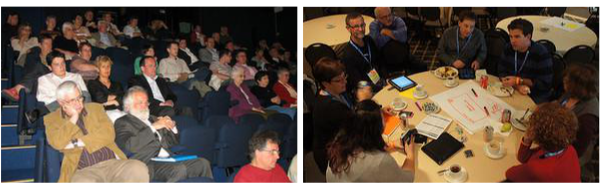
Day 2 at the SEG Annual Meeting in Las Vegas continued with 191 talks and dozens more posters. People are rushing around all over the place — there are absolutely no breaks, other than lunch, so it's easy to get frazzled. Here are my highlights:

Adam Halpert, Stanford

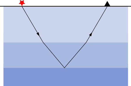
Image segmentation is an important class of problems in computer vision. An application to seismic data is to automatically pick a contiguous cloud of voxels from the 3D seismic image — a salt body, perhaps. Before trying to do this, it is common to reduce noise (e.g. roughness and jitter) by smoothing the image. The trick is to do this without blurring geologically important edges. Halpert did the hard work and assessed a number of smoothers for both efficacy and efficiency: median (easy), Kuwahara, maximum homogeneity median, Hale's bilateral [PDF], and AlBinHassan's filter. You can read all about his research in his paper online [PDF]. 

Dave Hale, Colorado School of Mines

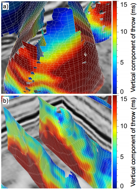
Automatic fault detection is a long-standing problem in interpretation. Methods tend to focus on optimizing a dissimilarity image of some kind (e.g. Bø 2012 and Dorn 2012), or on detecting planar discontinuities in that image. Hale's method is, I think, a new approach. And it seems to work well, finding fault planes and their throw (right).

Fear not, it's not complete automation — the method can't organize fault planes, interpret their meaning, or discriminate artifacts. But it is undoubtedly faster, more accurate, and more objective than a human. His test dataset is the F3 dataset from dGB's Open Seismic Repository. The shallow section, which resembles the famous polygonally faulted Eocene of the North Sea and elsewhere, contains point-up conical faults that no human would have picked. He is open to explanations of this geometry. 

Other good bits

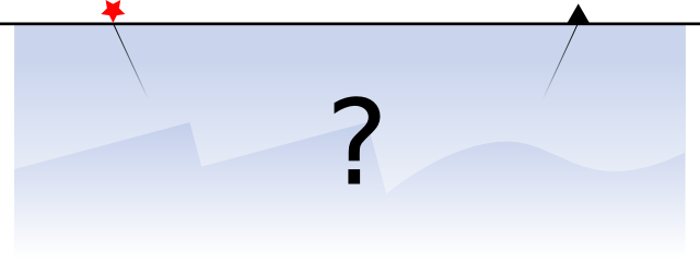
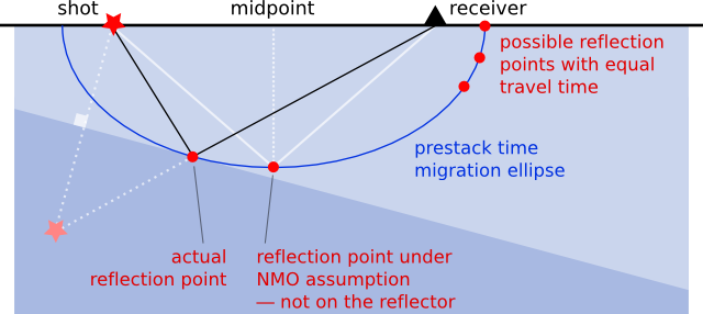
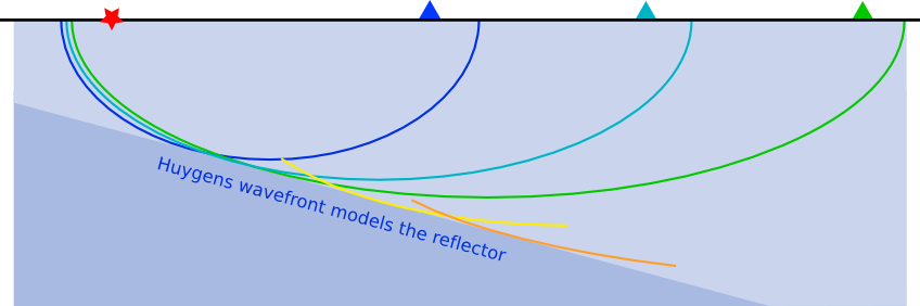
John Etgen and Chandan Kumar of BP made a very useful tutorial poster about the differences and similarities between pre-stack time and depth migration. They busted some myths about PreSTM:

  • Time migration is actually not always more amplitude-friendly than depth migration.
  • Time migration does not necessarily produce less noisy images.
  • Time migration does not necessarily produce higher frequency images.
  • Time migration is not necessarily less sensitive to velocity errors.
  • Time migration images do not necessarily have time units.
  • Time migrations can use the wave equation.
  • But time migration is definitely less expensive than depth migration. That's not a myth.

Brian Frehner of Oklahoma State presented his research [PDF] to the Historical Preservation Committee, which I happened to be in this morning. Check out his interesting-looking book, Finding Oil: The Nature of Petroleum Geology

Jon Claerbout of Stanford gave his first talk in several years. I missed it unfortunately, but Sergey Fomel said it was his highlight of the day, and that's good enough for me. Jon is a big proponent of openness in geophysics, so no surprise that he put his talk on YouTube days ago:

The image from Hale is copyright of SEG, from the 2012 Annual Meeting proceedings, and used here in accordance with their permissions guidelines. The DOI links in this post don't work at the time of writing — SEG is on it. 

Resolution, anisotropy, and brains

Day 1 of the SEG Annual Meeting continued with the start of the regular program — 96 talks and 71 posters, not to mention the 323 booths on the exhibition floor. Instead of deciding where to start, I wandered around the bookstore and bought Don Herron's nice-looking new book, First Steps in Seismic Interpretation, which we will review some time soon.

Here are my highlights from the rest of the day.

Chuck Ursenbach, Arcis

Calgary is the home of seismic geophysics. There's a deep tradition of signal processing, and getting the basics right. Sometimes there's snake oil too, but mostly it's good, honest science. And mathematics. So when Jim Gaiser suggested last year at SEG that PS data might offer as good resolution as SS or PP — as good, and possibly better — you know someone in Calgary will jump on it with MATLAB. Ursenbach, Cary, and Perz [PDF] did some jumping, and conclude: PP-to-PS mapping can indeed increase bandwidth, but the resolution is unchanged, because the wavelength is unchanged — 'conservation of resolution', as Ursenbach put it. Resolution isn't everything. 

Gabriel Chao, Total E&P

Chao showed a real-world case study starting with a PreSTM gather with a decent Class 2p AVO anomaly at the top of the reservoir interval (TTI Kirchhoff with 450–4350 m offset). There was residual NMO in the gather, as Leon Thomsen himself later forced Chao to admit, but there did seem to be a phase reversal at about 25°. The authors compared the gather with three synthetics: isotropic convolutional, anisotropic convolutional, and full waveform. The isotropic model was fair, but the phase reversal was out at 33°. The anisotropic convolutional model matched well right up to about 42°, beyond which only the full waveform model was close (right). Anisotropy made a similar difference to wavelet extraction, especially beyond about 25°.

Canada prevails

With no hockey to divert them, Canadians are focusing on geophysical contests this year. With the Canadian champions Keneth Silva and Abdolnaser Yousetz Zadeh denied the chance to go for the world title by circumstances beyond their control, Canada fielded a scratch team of Adrian Smith (U of C) and Darragh O'Connor (Dalhousie). So much depth is there in the boreal Americas that the pair stormed home with the trophy, the cash, and the glory.

The Challenge Bowl event was a delight — live music, semi-raucous cheering, and who can resist MC Peter Duncan's cheesy jests? If you weren't there, promise yourself you'll go next year. 

The image from Chao is copyright of SEG, from the 2012 Annual Meeting proceedings, and used here in accordance with their permissions guidelines. The image of Herron's book is also copyright of SEG; its use here is proposed to be fair use.

Ways to experiment with conferences

Yesterday I wrote about why I think technical conferences underdeliver. Coincidentally, Evan sent me this quote from Seth Godin's blog yesterday:

We've all been offered access to so many tools, so many valuable connections, so many committed people. What an opportunity.

What should we do about it? 

If we are collectively spending 6 careers at the SEG Annual Meeting every autumn, as I asserted yesterday, let's put some of that cognitive surplus to work!

I suggest starting to experiment with our conferences. There are so many tools: unconferences, idea jams, hackdays, wikithons, and other participative activities. Anything to break up sitting in the dark watching 16 lectures a day, slamming coffee and cramming posters in between. Anything to get people not just talking and drinking, but working together. What a way to build collaborations, friendships, and trust. Connecting with humans, not business cards. 

Unconvinced? consider which of these groups of people looks like they're learning, being productive, and having fun:

This year I've been to some random (for me) conferences — Science Online, Wikimania, and Strata. Here are some engaging, fun, and inspiring things happening in meetings of those communities:

  • Speaker 'office hours' during the breaks so you can find them and ask questions. 
  • Self-selected topical discussion tables at lunch. 
  • Actual time for actual discussion after talks (no, really!).
  • Cool giveaways: tattoos and stickers, funky notebooks, useful mobile apps, books, scientific toys.
  • A chance to sit down and work with others — hackathons, co-writing, idea jams, and so on. 
  • Engaged, relevant, grounded social media presence, not more marketing.
  • An art gallery, including graphics captured during sessions
  • No posters! Those things epitomize the churn of one-way communication.

Come to our experiment!

Clearly there's no shortage of things to try. Converting a session here, a workshop there — it's easy to do something in a sandbox, alongside the traditional. And by 'easy', I mean uncertain, risky and uncomfortable. It will require a new kind of openness. I'm not certain of the outcome, but I am certain that it's worth doing. 

On this note, a wonderful thing happened to us recently. We were — and still are — planning an unconference of our own (stay tuned for that). Then, quite unprovoked, Carmen Dumitrescu asked Evan if we'd like to chair a session at the Canada GeoConvention in May. And she invited us to 'do something different'. Perfect timing!

So — mark your calendar! GeoConvention, Calgary, May 2013. Something different.

The photo of the lecture, from the depressing point of view of the speaker, is licensed CC-BY-SA by Flickr user Pierre-Alain Dorange. The one of the unconference is licensed CC-BY-SA-NC by Flickr user aforgrave.

Are conferences failing you too?

I recently asked a big software company executive if big exhibitions are good marketing value. The reply:

It's not a waste of money. It's a colossal waste of money.

So that's a 'no'.

Is there a problem here?

Next week I'll be at the biggest exhibition (and conference) in our sector: the SEG Annual Meeting. Thousands of others will be there, but far more won’t. Clearly it’s not indispensable or unmissable. Indeed, it’s patently missable — I did just fine in my career as a geophysicist without ever going. Last year was my first time.

Is this just the nature of mass market conferences? Is the traditional academic format necessarily unremarkable? Do the technical societies try too hard to be all things to all people, and thereby miss the mark for everyone? 

I don't know the answer to any of these questions, I can only speak for myself. I'm getting tired of conferences. Perhaps I've reached some new loop in the meandering of my career, or perhaps I'm just grumpy. But as I've started to whine, I'm finding more and more allies in my conviction that conferences aren't awesome.

What are conferences for?

  • They make lots of money for the technical societies that organize them.
  • A good way to do this is to provide marketing and sales opportunities for the exhibiting vendors.
  • A good way to do this is to attract lots of scientists there, baiting with talks by all the awesomest ones.
  • A good way to do this, apparently, is to hold it in Las Vegas.

But I don't think the conference format is great at any of these things, except possibly the first one. The vendors get prospects (that's what sales folk call people) that are only interested in toys and beer — they might be users, but they aren't really customers. The talks are samey and mostly not memorable (and you can only see 5% of them). Even the socializing is limited by the fact that the conference is gigantic and run on a tight schedule. And don't get me started on Las Vegas. 

If we're going to take the trouble of flying 8000 people to Las Vegas, we had better have something remarkable to show for it. Do we? What do we get from this giant conference? By my conservative back-of-the-envelope calculation, we will burn through about 210 person-years of productivity in Las Vegas next week. That's about 6 careers' worth. Six! Are we as a community satisfied that we will produce 6 careers' worth of insight, creativity, and benefit?

You can probably tell that I am not convinced. Tomorrow, I will put away the wrecking ball of bellyaching, and offer some constructive ideas, and a promise. Meanwhile, if you have been to an amazing conference, or can describe one from your imagination, or think I'm just being a grouch — please use the comments below.

Map data ©2012 Google, INEGI, MapLink, Tele Atlas. 

N is for Nyquist

In yesterday's post, I covered a few ideas from Fourier analysis for synthesizing and processing information. It serves as a primer for the next letter in our A to Z blog series: N is for Nyquist.

In seismology, the goal is to propagate a broadband impulse into the subsurface, and measure the reflected wavetrain that returns from the series of rock boundaries. A question that concerns the seismic experiment is: What sample rate should I choose to adequately capture the information from all the sinusoids that comprise the waveform? Sampling is the capturing of discrete data points from the continuous analog signal — a necessary step in recording digital data. Oversample it, using too high a sample rate, and you might run out of disk space. Undersample it and your recording will suffer from aliasing.

What is aliasing?

Aliasing is a phenomenon observed when the sample interval is not sufficiently brief to capture the higher range of frequencies in a signal. In order to avoid aliasing, each constituent frequency has to be sampled at least two times per wavelength. So the term Nyquist frequency is defined as half of the sampling frequency of a digital recording system. Nyquist has to be higher than all of the frequencies in the observed signal to allow perfect recontstruction of the signal from the samples.

Above Nyquist, the signal frequencies are not sampled twice per wavelength, and will experience a folding about Nyquist to low frequencies. So not obeying Nyquist gives a double blow, not only does it fail to record all the frequencies, the frequencies that you leave out actually destroy part of the frequencies you do record. Can you see this happening in the seismic reflection trace shown below? You may need to traverse back and forth between the time domain and frequency domain representation of this signal.

Nyquist_trace.png

Seismic data is usually acquired with either a 4 millisecond sample interval (250 Hz sample rate) if you are offshore, or 2 millisecond sample interval (500 Hz) if you are on land. A recording system with a 250 Hz sample rate has a Nyquist frequency of 125 Hz. So information coming in above 150 Hz will wrap around or fold to 100 Hz, and so on. 

It's important to note that the sampling rate of the recording system has nothing to do the native frequencies being observed. It turns out that most seismic acquisition systems are safe with Nyquist at 125 Hz, because seismic sources such as Vibroseis and dynamite don't send high frequencies very far; the earth filters and attenuates them out before they arrive at the receiver.

Space alias

Aliasing can happen in space, as well as in time. When the pixels in this image are larger than half the width of the bricks, we see these beautiful curved artifacts. In this case, the aliasing patterns are created by the very subtle perspective warping of the curved bricks across a regularly sampled grid of pixels. It creates a powerful illusion, a wonderful distortion of reality. The observations were not sampled at a high enough rate to adequately capture the nature of reality. Watch for this kind of thing on seismic records and sections. Spatial alaising. 

Click for the full demonstration (or adjust your screen resolution).You may also have seen this dizzying illusion of an accelerating wheel that suddenly appears to change direction after it rotates faster than the sample rate of the video frames captured. The classic example is the wagon whel effect in old Western movies.

Aliasing is just one phenomenon to worry about when transmitting and processing geophysical signals. After-the-fact tricks like anti-aliasing filters are sometimes employed, but if you really care about recovering all the information that the earth is spitting out at you, you probably need to oversample. At least two times for the shortest wavelengths.

The blind geoscientist

Last time I wrote about using randomized, blind, controlled tests in geoscience. Today, I want to look a bit closer at what such a test or experiment might look like. But before we do anything else, it's worth taking 20 minutes, or at least 4, to watch Ben Goldacre's talk on the subject at Strata in London recently:

How would blind testing work?

It doesn't have to be complicated, or much different from what you already do. Here’s how it could work for the biostrat study I mentioned last time:

  1. Collect the samples as normal. There is plenty of nuance here too: do you sample regularly, or do you target ‘interesting’ zones? Only regular sampling is free from bias, but it’s expensive.
  2. Label the samples with unique identifiers, perhaps well name and depth.
  3. Give the samples to a disinterested, competent person. They repackage the samples and assign different identifiers randomly to the samples.
  4. Send the samples for analysis. Provide no other data. Ask for the most objective analysis possible, without guesswork about sample identification or origin. The samples should all be treated in the same way.
  5. When you get the results, analyse the data for quality issues. Perform any analysis that does not depend on depth or well location — for example, cluster analysis.
  6. If you want to be really thorough, the disinterested party to provide depths only, allowing you to sort by well and by depth but without knowing which wells are which. Perform any analysis that doesn’t depend on spatial location.
  7. Finally, ask for the key that reveals well names. Hopefully, any problems with the data have already revealed themselves. At this point, if something doesn’t fit your expectations, maybe your expectations need adjusting!

Where else could we apply these ideas?

  1. Random selection of some locations in a drilling program, perhaps in contraindicated locations
  2. Blinded, randomized inspection of gathers, for example with different processing parameters
  3. Random selection of wells as blind control for a seismic inversion or attribute analysis
  4. Random selection of realizations from geomodel simulation, for example for flow simulation
  5. Blinded inspection of the results of a 'turkey shoot' or vendor competition (e.g. Hayles et al, 2011)

It strikes me that we often see some of this — one or two wells held back for blind testing, or one well in a program that targets a non-optimal location. But I bet they are rarely selected randomly (more like grudgingly), and blind samples are often peeked at ('just to be sure'). It's easy to argue that "this is a business, not a science experiment", but that's fallacious. It's because it's a business that we must get the science right. Scientific rigour serves the business.

I'm sure there are dozens of other ways to push in this direction. Think about the science you're doing right now. How could you make it a little less prone to bias? How can you make it a shade less likely that you'll pull the wool over your own eyes?

Experimental good practice

Like hitting piñatas, scientific experiments need blindfolds. Image: Juergen. CC-BY.I once sent some samples to a biostratigrapher, who immediately asked for the logs to go with the well. 'Fair enough,' I thought, 'he wants to see where the samples are from'. Later, when we went over the results, I asked about a particular organism. I was surprised it was completely absent from one of the samples. He said, 'oh, it’s in there, it’s just not important in that facies, so I don’t count it.' I was stunned. The data had been interpreted before it had even been collected.

I made up my mind to do a blind test next time, but moved to another project before I got the chance. I haven’t ordered lab analyses since, so haven't put my plan into action. To find out if others already do it, I asked my Twitter friends:

Randomized, blinded, controlled testing should be standard practice in geoscience. I mean, if you can randomize trials of government policy, then rocks should be no problem. If there are multiple experimenters involved, like me and the biostrat guy in the story above, perhaps there’s an argument for double-blinding too.

Designing a good experiment

What should we be doing to make geoscience experiments, and the reported results, less prone to bias and error? I'm no expert on lab procedure, but for what it's worth, here are my seven Rs:

  • Randomized blinding or double-blinding. Look for opportunities to fight confirmation bias. There’s some anecdotal evidence that geochronologists do this, at least informally — can you do it too, or can you do more?
  • Regular instrument calibration, per manufacturer instructions. You should be doing this more often than you think you need to do it.
  • Repeatability tests. Does your method give you the same answer today as yesterday? Does an almost identical sample give you the same answer? Of course it does! Right? Right??
  • Report errors. Error estimates should be based on known problems with the method or the instrument, and on the outcomes of calibration and repeatability tests. What is the expected variance in your result?
  • Report all the data. Unless you know there was an operational problem that invalidated an experiment, report all your data. Don’t weed it, report it. 
  • Report precedents. How do your results compare to others’ work on the same stuff? Most academics do this well, but industrial scientists should report this rigorously too. If your results disagree, why is this? Can you prove it?
  • Release your data. Follow Hjalmar Gislason's advice — use CSV and earn at least 3 Berners-Lee stars. And state the license clearly, preferably a copyfree one. Open data is not altruistic — it's scientific.

Why go to all this trouble? Listen to Richard Feynman:

The first principle is that you must not fool yourself, and you are the easiest person to fool.

Thank you to @ToriHerridge@mammathus@volcan01010 and @ZeticaLtd for the stories about blinded experiments in geoscience. There are at least a few out there. Do you know of others? Have you tried blinding? We'd love to hear from you in the comments! 

M is for Migration

One of my favourite phrases in geophysics is the seismic experiment. I think we call it that to remind everyone, especially ourselves, that this is science: it's an experiment, it will yield results, and we must interpret those results. We are not observing anything, or remote sensing, or otherwise peering into the earth. When seismic processors talk about imaging, they mean image construction, not image capture

The classic cartoon of the seismic experiment shows flat geology. Rays go down, rays refract and reflect, rays come back up. Simple. If you know the acoustic properties of the medium—the speed of sound—and you know the locations of the source and receiver, then you know where a given reflection came from. Easy!

But... some geologists think that the rocks beneath the earth's surface are not flat. Some geologists think there are tilted beds and faults and big folds all over the place. And, more devastating still, we just don't know what the geometries are. All of this means trouble for the geophysicist, because now the reflection could have come from an infinite number of places. This makes choosing a finite number of well locations more of a challenge. 

What to do? This is a hard problem. Our solution is arm-wavingly called imaging. We wish to reconstruct an image of the subsurface, using only our data and our sharp intellects. And computers. Lots of those.

Imaging with geometry

Agile's good friend Brian Russell wrote one of my favourite papers (Russell, 1998) — an imaging tutorial. Please read it (grab some graph paper first). He walks us through a simple problem: imaging a single dipping reflector.

Remember that in the seismic experiment, all we know is the location of the shots and receivers, and the travel time of a sound wave from one to the other. We do not know the reflection points in the earth. If we assume dipping geology, we can use the NMO equation to compute the locus of all possible reflection points, because we know the travel time from shot to receiver. Solutions to the NMO equation — given source–receiver distance, travel time, and the speed of sound — thus give the ellipse of possible reflection points, shown here in blue:

Clearly, knowing all possible reflection points is interesting, but not very useful. We want to know which reflection point our recorded echo came from. It turns out we can do something quite easy, if we have plenty of data. Fortunately, we geophysicists always bring lots and lots of receivers along to the seismic experiment. Thousands usually. So we got data.

Now for the magic. Remember Huygens' principle? It says we can imagine a wavefront as a series of little secondary waves, the sum of which shows us what happens to the wavefront. We can apply this idea to the problem of the tilted bed. We have lots of little wavefronts — one for each receiver. Instead of trying to figure out the location of each reflection point, we just compute all possible reflection points, for all receivers, then add them all up. The wavefronts add constructively at the reflector, and we get the solution to the imaging problem. It's kind of a miracle. 

Try it yourself. Brian Russell's little exercise is (geeky) fun. It will take you about an hour. If you're not a geophysicist, and even if you are, I guarantee you will learn something about how the miracle of the seismic experiment. 

Reference
Russell, B (1998). A simple seismic imaging exercise. The Leading Edge 17 (7), 885–889. DOI: 10.1190/1.1438059

L is for Lambda

Hooke's law says that the force F exerted by a spring depends only on its displacement x from equilibrium, and the spring constant k of the spring:

.

We can think of k—and experience it—as stiffness. The spring constant is a property of the spring. In a sense, it is the spring. Rocks are like springs, in that they have some elasticity. We'd like to know the spring constant of our rocks, because it can help us predict useful things like porosity. 

Hooke's law is the basis for elasticity theory, in which we express the law as

stress [force per unit area] is equal to strain [deformation] times a constant

This time the constant of proportionality is called the elastic modulus. And there isn't just one of them. Why more complicated? Well, rocks are like springs, but they are three dimensional.

In three dimensions, assuming isotropy, the shear modulus μ plays the role of the spring constant for shear waves. But for compressional waves we need λ+2μ, a quantity called the P-wave modulus. So λ is one part of the term that tells us how rocks get squished by P-waves.

These mysterious quantities λ and µ are Lamé's first and second parameters. They are intrinsic properties of all materials, including rocks. Like all elastic moduli, they have units of force per unit area, or pascals [Pa].

So what is λ?

Matt and I have spent several hours discussing how to describe lambda. Unlike Young's modulus E, or Poisson's ratio ν, our friend λ does not have a simple physical description. Young's modulus just determines how much longer something gets when I stretch it. Poisson's ratio tells how much fatter something gets if I squeeze it. But lambda... what is lambda?

  • λ is sometimes called incompressibility, a name best avoided because it's sometimes also used for the bulk modulus, K.  
  • If we apply stress σ1 along the 1 direction to this linearly elastic isotropic cube (right), then λ represents the 'spring constant' that scales the strain ε along the directions perpendicular to the applied stress.
  • The derivation of Hooke's law in 3D requires tensors, which we're not getting into here. The point is that λ and μ help give the simplest form of the equations (right, shown for one dimension).

The significance of elastic properties is that they determine how a material is temporarily deformed by a passing seismic wave. Shear waves propagate by orthogonal displacements relative to the propagation direction—this deformation is determined by µ. In contrast, P-waves propagate by displacements parallel to the propagation direction, and this deformation is inversely proportional to M, which is 2µ + λ

Lambda rears its head in seismic petrophysics, AVO inversion, and is the first letter in the acronym of Bill Goodway's popular LMR inversion method (Goodway, 2001). Even though it is fundamental to seismic, there's no doubt that λ is not intuitively understood by most geoscientists. Have you ever tried to explain lambda to someone? What description of λ do you find useful? I'm open to suggestions. 

Goodway, B., 2001, AVO and Lame' constants for rock parameterization and fluid detection: CSEG Recorder, 26, no. 6, 39-60.

Cross plots: a non-answer

On Monday I asked whether we should make crossplots according to statistical rules or natural rules. There was some fun discussion, and some awesome computation from Henry Herrera, and a couple of gems:

Physics likes math, but math doesn't care about physics — @jeffersonite

But... when I consider the intercept point I cannot possibly imagine a rock that has high porosity and zero impedance — Matteo Niccoli, aka @My_Carta

I tried asking on Stack Overflow once, but didn’t really get to the bottom of it, or perhaps I just wasn't convinced. The consensus seems to be that the statistical answer is to put porosity on y-axis, because that way you minimize the prediction error on porosity. But I feel—and this is just my flaky intuition talking—like this fails to represent nature (whatever that means) and so maybe that error reduction is spurious somehow.

Reversing the plot to what I think of as the natural, causation-respecting plot may not be that unreasonable. It's effectively the same as reducing the error on what was x (that is, impedance), instead of y. Since impedance is our measured data, we could say this regression respects the measured data more than the statistical, non-causation-respecting plot.

So must we choose? Minimize the error on the prediction, or minimize the error on the predictor. Let's see. In the plot on the right, I used the two methods to predict porosity at the red points from the blue. That is, I did the regression on the blue points; the red points are my blind data (new wells, perhaps). Surprisingly, the statistical method gives an RMS error of 0.034, the natural method 0.023. So my intuition is vindicated! 

Unfortunately if I reverse the datasets and instead model the red points, then predict the blue, the effect is also reversed: the statistical method does better with 0.029 instead of 0.034. So my intuition is wounded once more, and limps off for an early bath.

Irreducible error?

Here's what I think: there's an irreducible error of prediction. We can beg, borrow or steal error from one variable, but then it goes on the other. It's reminiscent of Heisenberg's uncertainty principle, but in this case, we can't have arbitrarily precise forecasts from imperfectly correlated data. So what can we do? Pick a method, justify it to yourself, test your assumptions, and then be consistent. And report your errors at every step. 

I'm reminded of the adage 'Correlation does not equal causation.' Indeed. And, to borrow @jeffersonite's phrase, it seems correlation also does not care about causation.