TRANSFORM happened!

How do you describe the indescribable?

Last week, Agile hosted the TRANSFORM unconference in Normandy, France. We were there to talk about the open suburface stack — the collection of open-source Python tools for earth scientists. We also spent time on the state of the Software Underground, a global community of practice for digital subsurface scientists and engineers. In effect, this was the first annual Software Underground conference. This was SwungCon 1.

The space

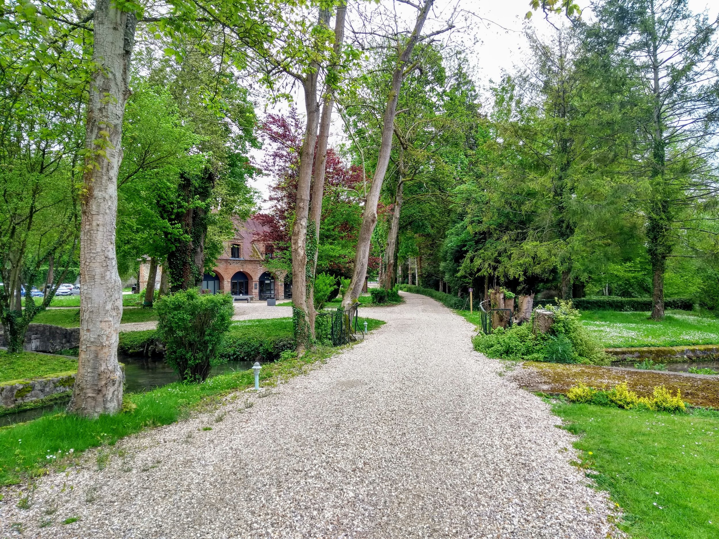
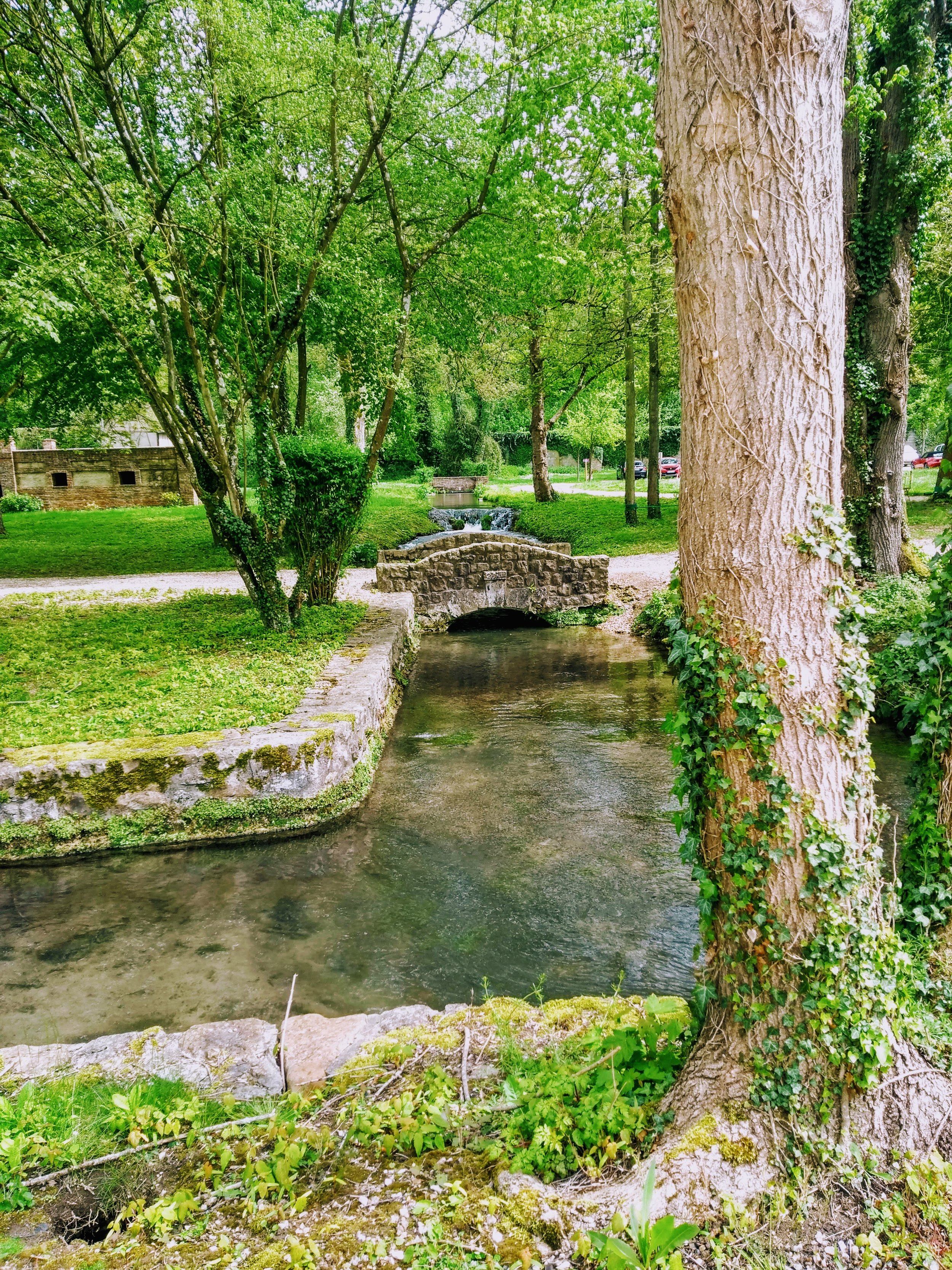
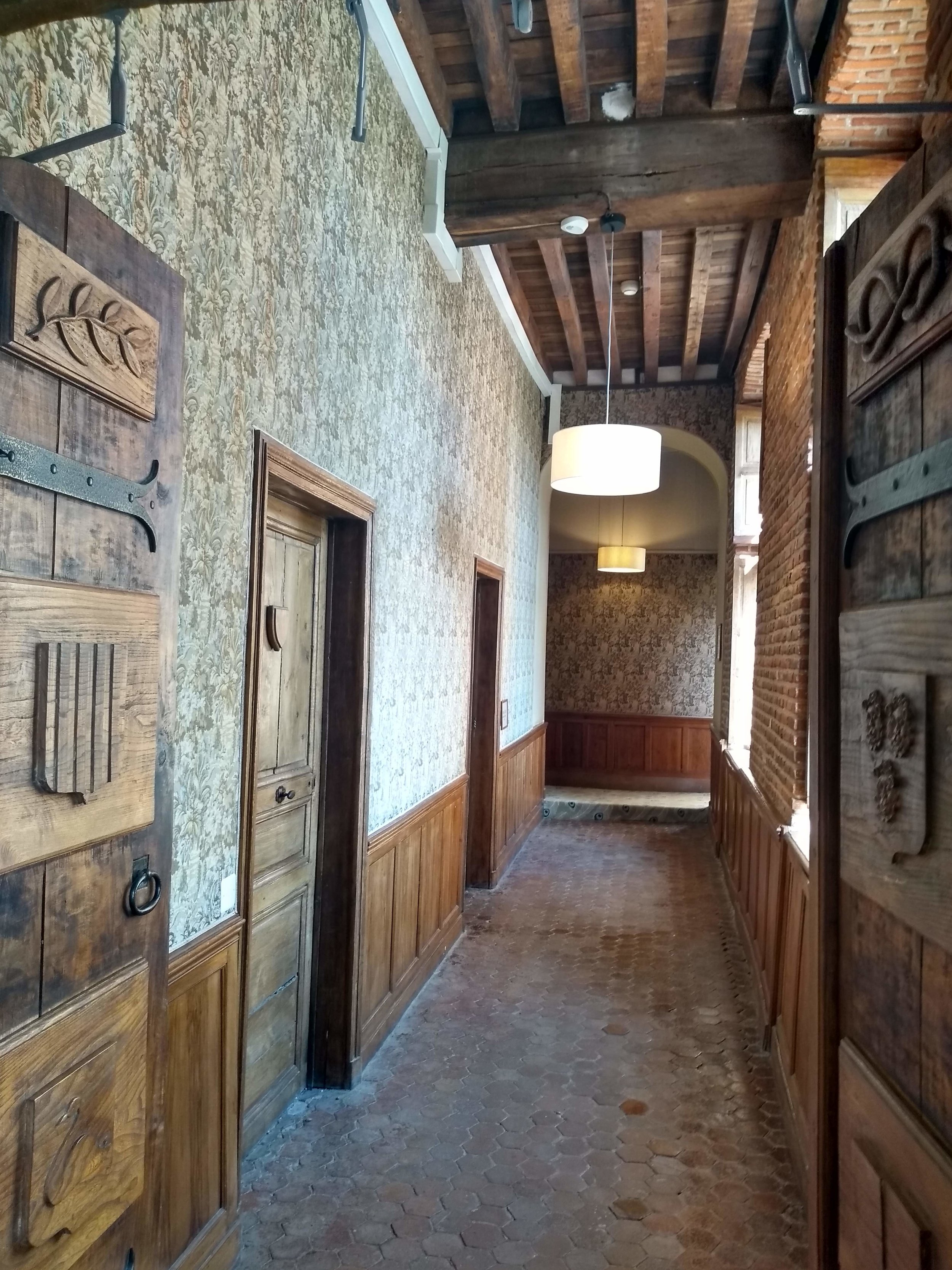
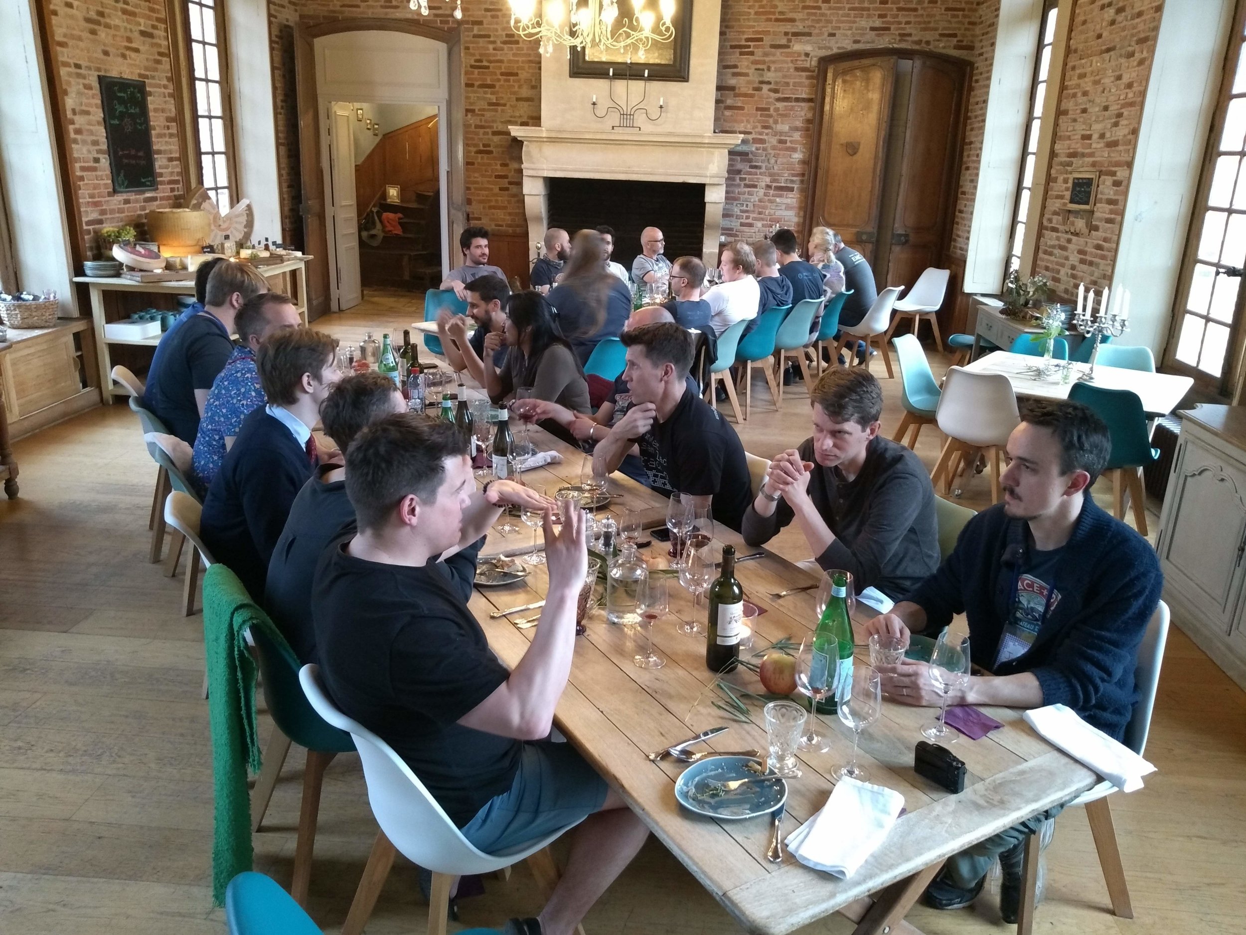
I knew the Château de Rosay was going to be nice. I hoped it was going to be very nice. But it wasn’t either of those things. It exceeded expectations by such a large margin, it seemed a little… indulgent, Excessive even. And yet it was cheaper than a Hilton, and you couldn’t imagine a more perfect place to think and talk about the future of open source geoscience, or a more productive environment in which to write code with new friends and colleagues.

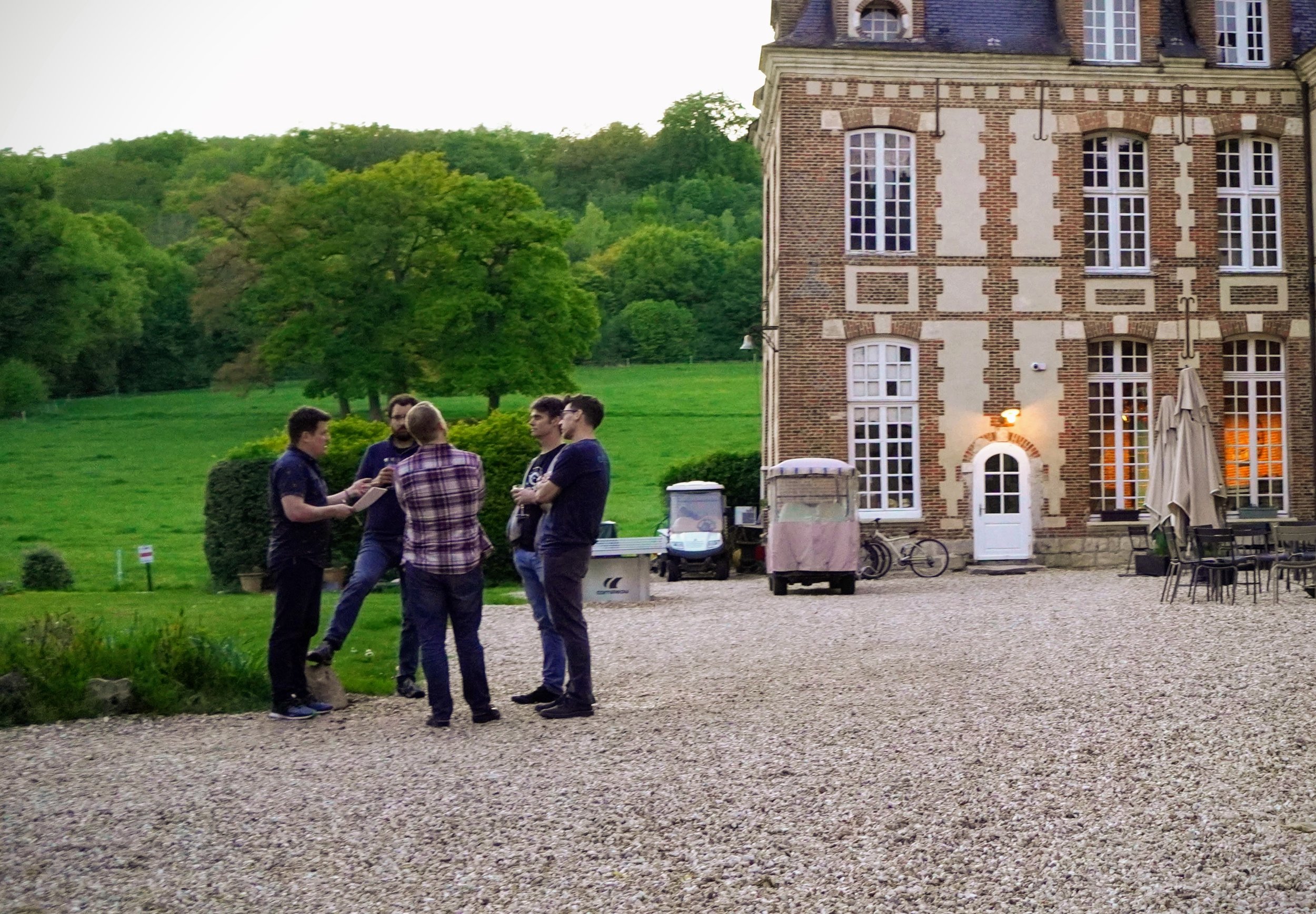
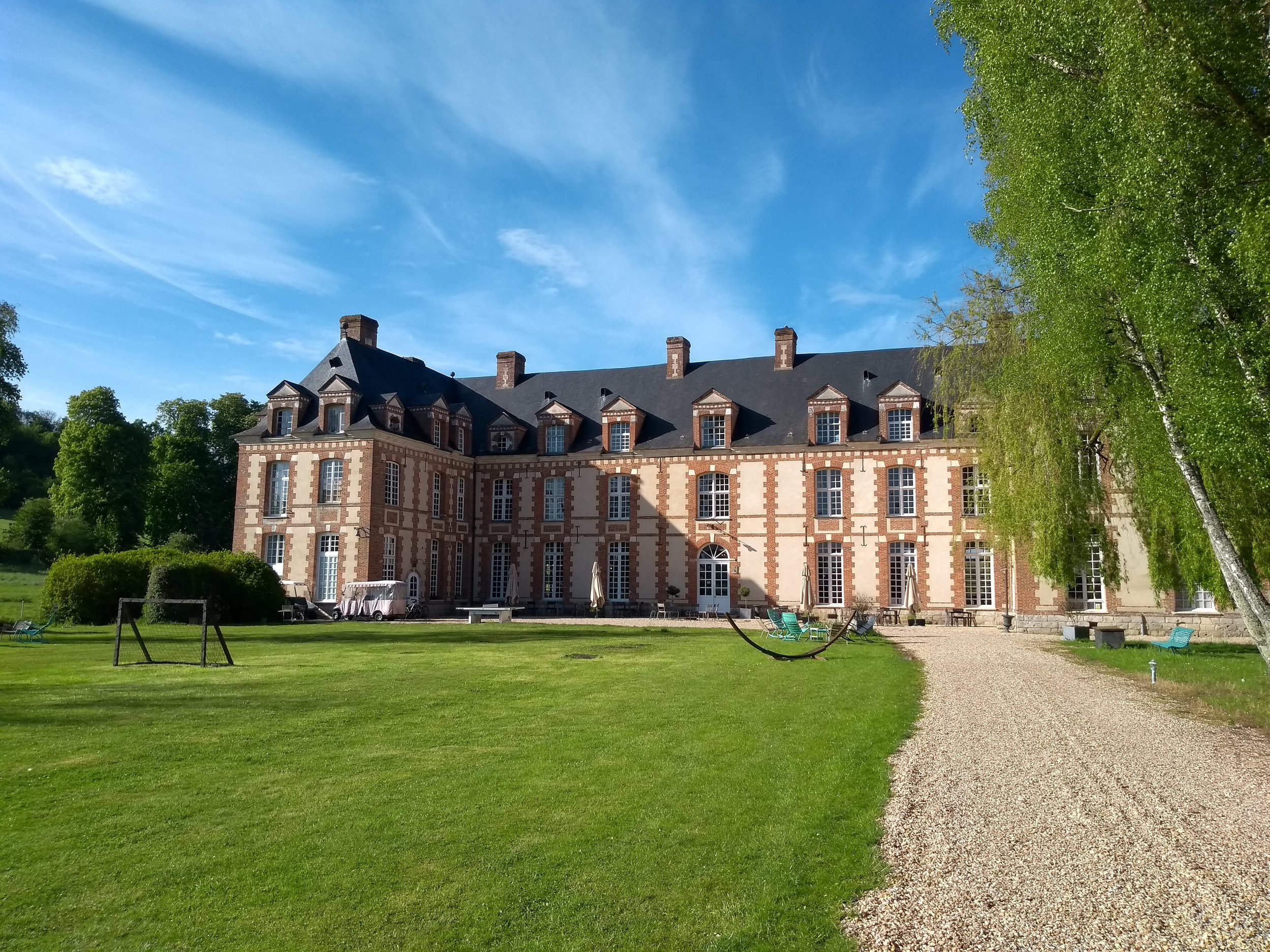
It turns out that a 400-year-old château set in 8 acres of parkland in the heart of Normandy is a great place to create new things. I expect Gustave Flaubert and Guy de Maupassant thought the same when they stayed there 150 years ago. The forty-two bedrooms house exactly the right number of people for a purposeful scientific meeting.

This is frustrating, I’m not doing the place justice at all.

The work

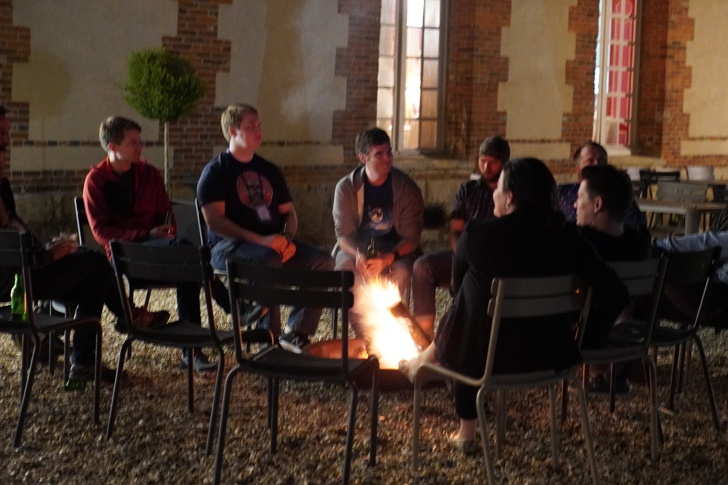
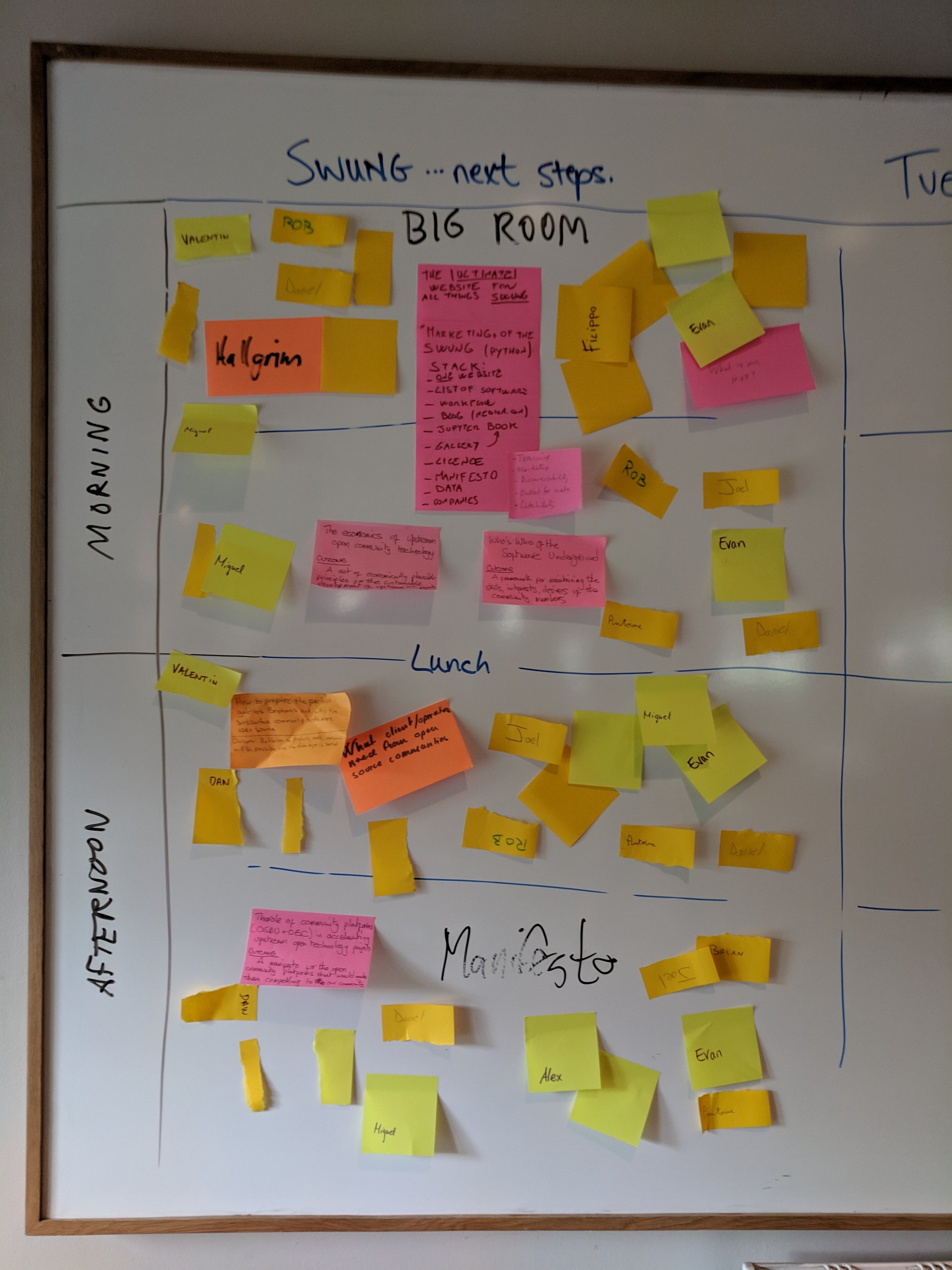
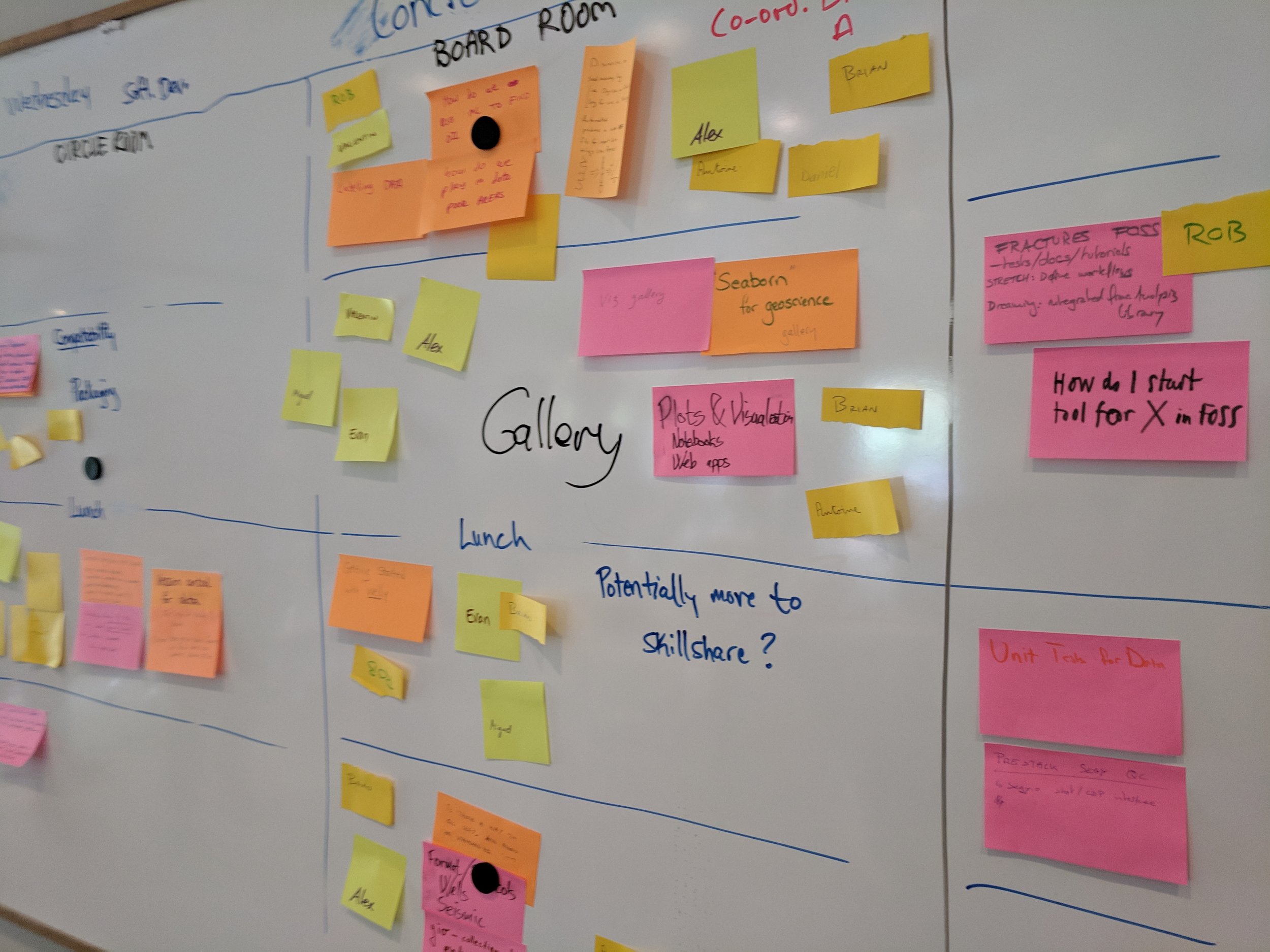
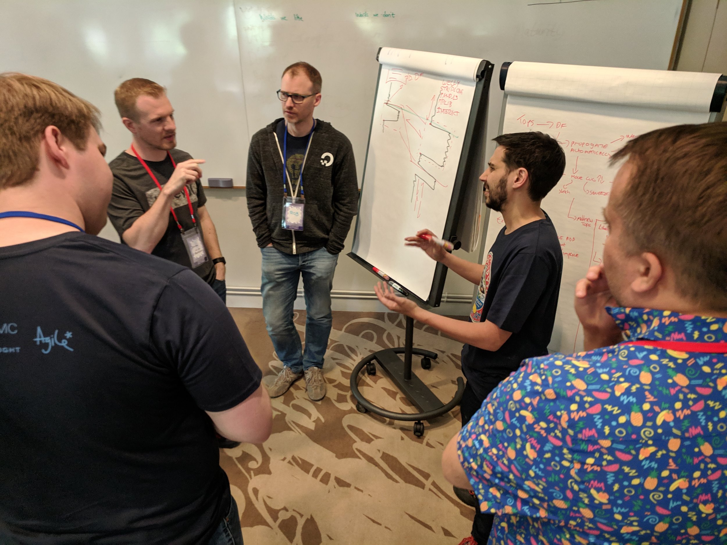
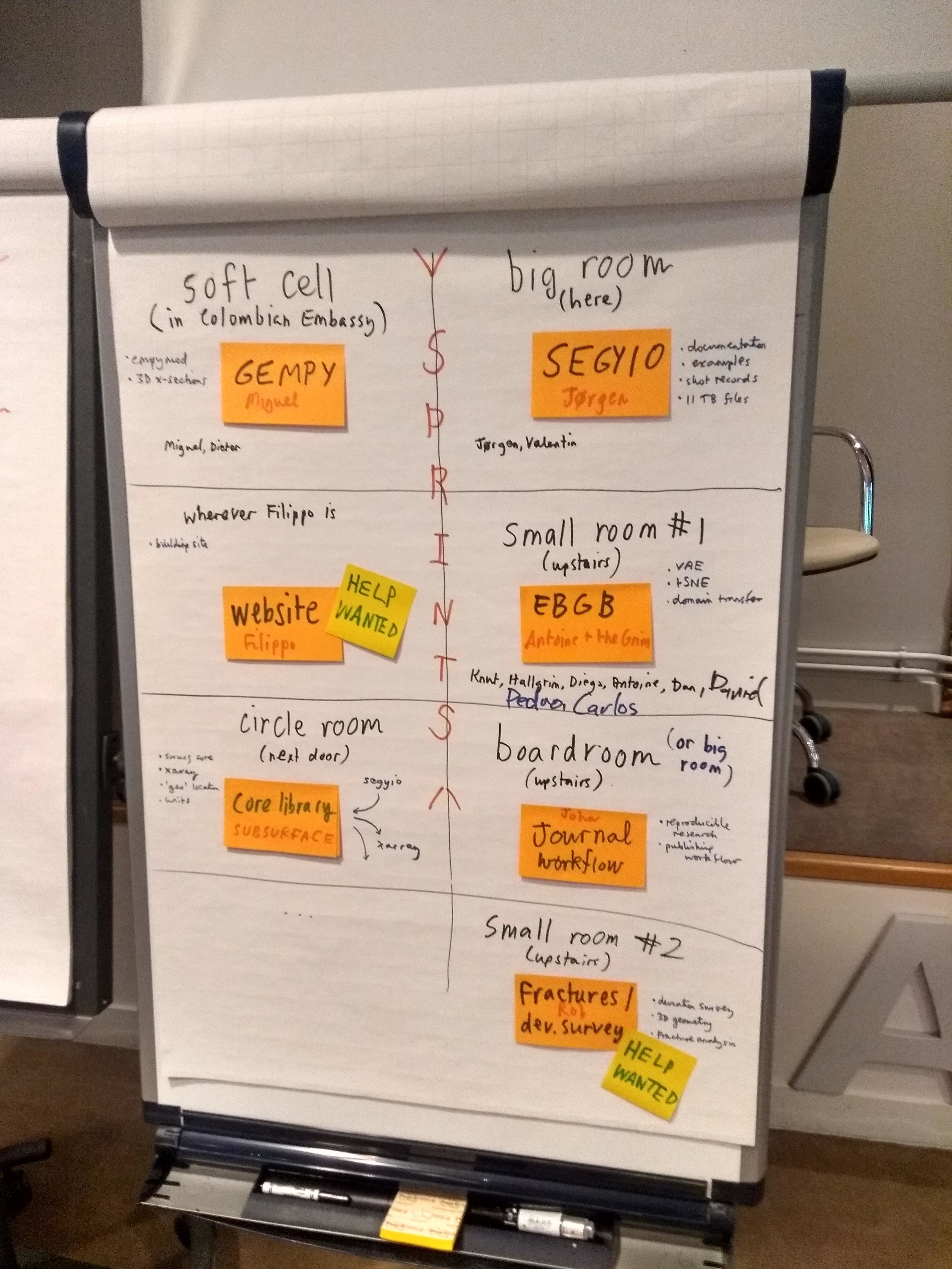
This was most people’s first experience of an unconference. It was undeniably weird walking into a week-long meeting with no schedule of events. But, despite being inexpertly facilitated by me, the 26 participants enthusiastically collaborated to create the agenda on the first morning. With time, we appreciated the possibilities of the open space — it lets the group talk about exactly what it needs to talk about, exactly when it needs to talk about it.

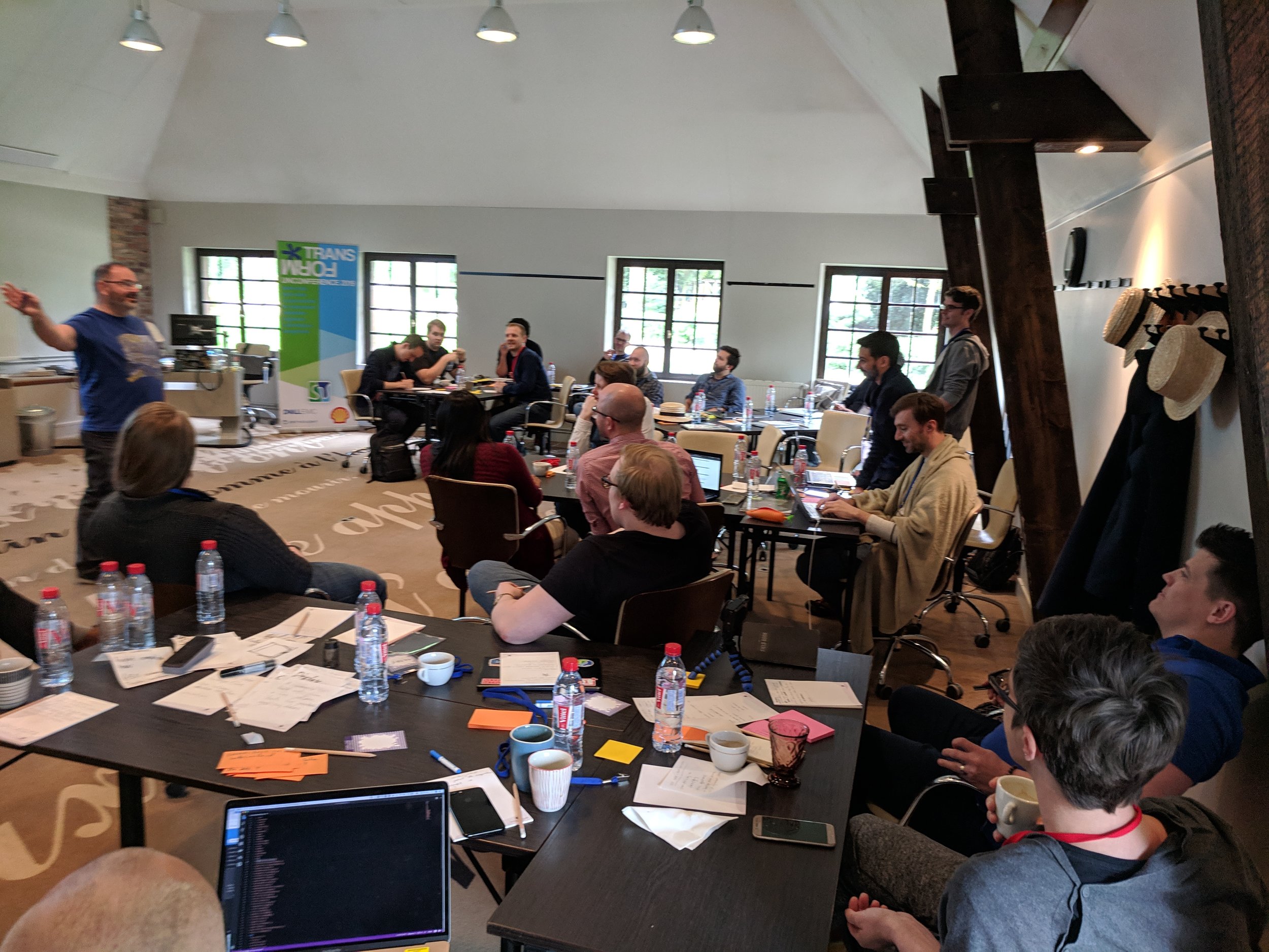
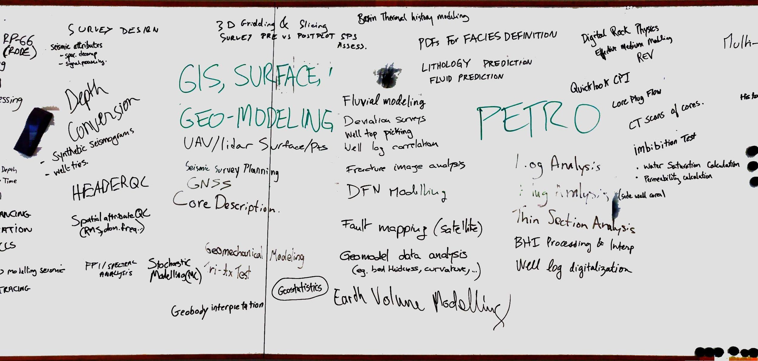
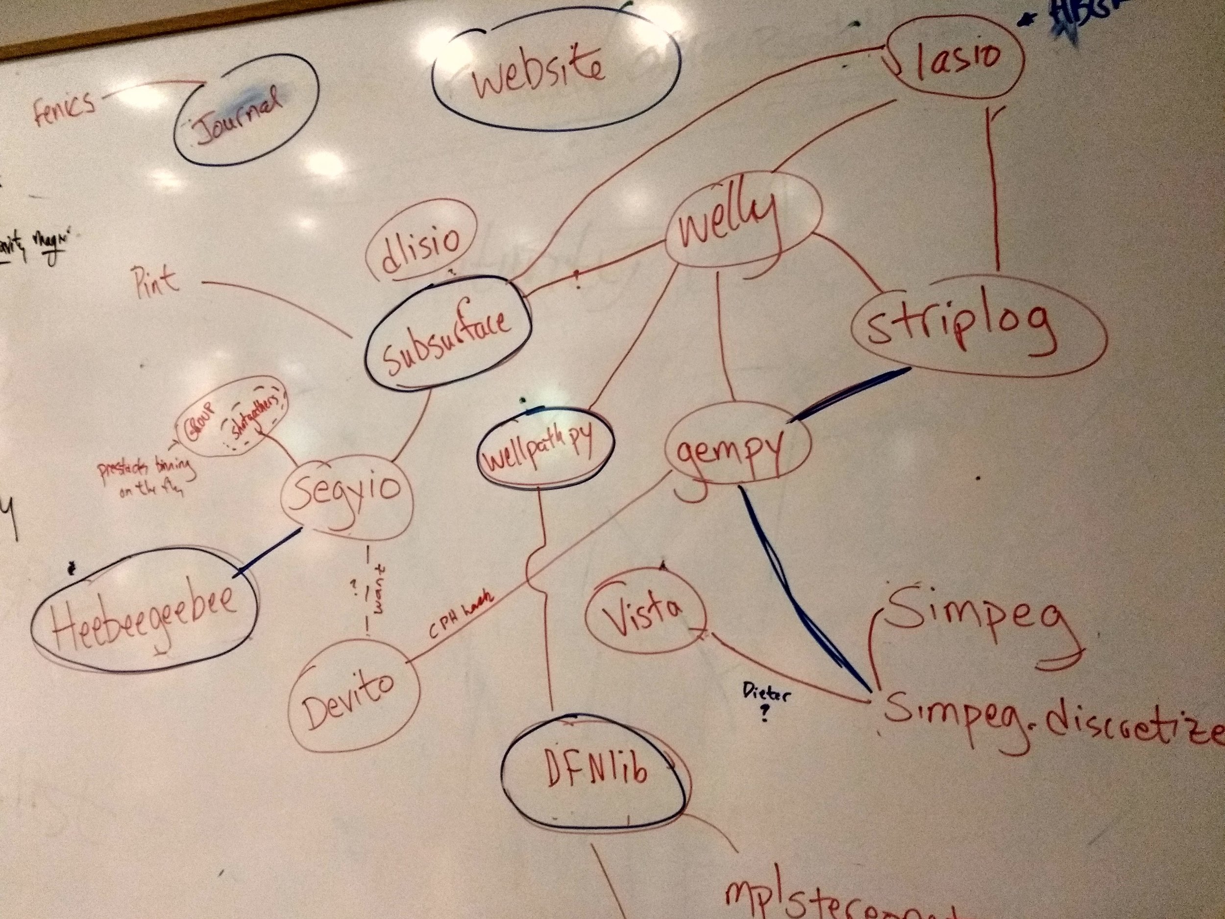
The topics ranged from the governance and future of the Software Underground, to the possibility of a new open access journal, interesting new events in the Software Underground calendar, new libraries for geoscience, a new ‘core’ library for wells and seismic, and — of course — machine learning. I’ll be writing more about all of these topics in the coming weeks, and there’s already lots of chatter about them on the Software Underground Slack (which hit 1500 members yesterday!).

The food

I can’t help it. I have to talk about the food.

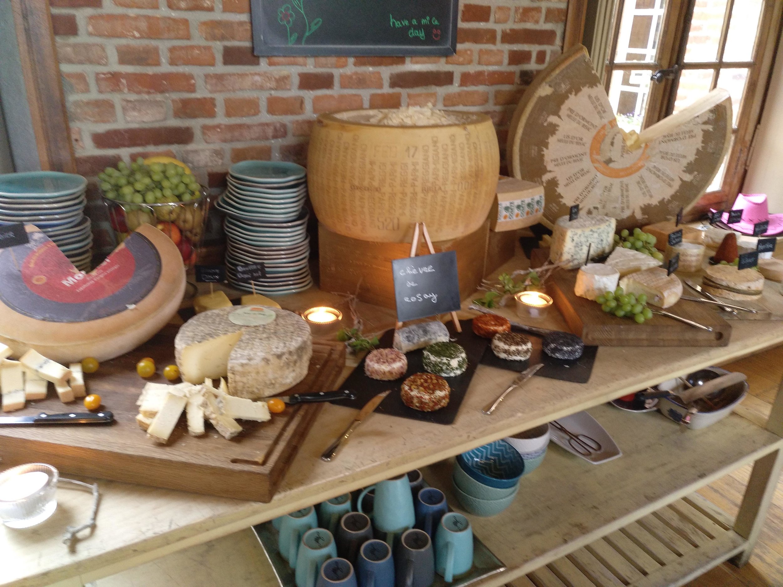
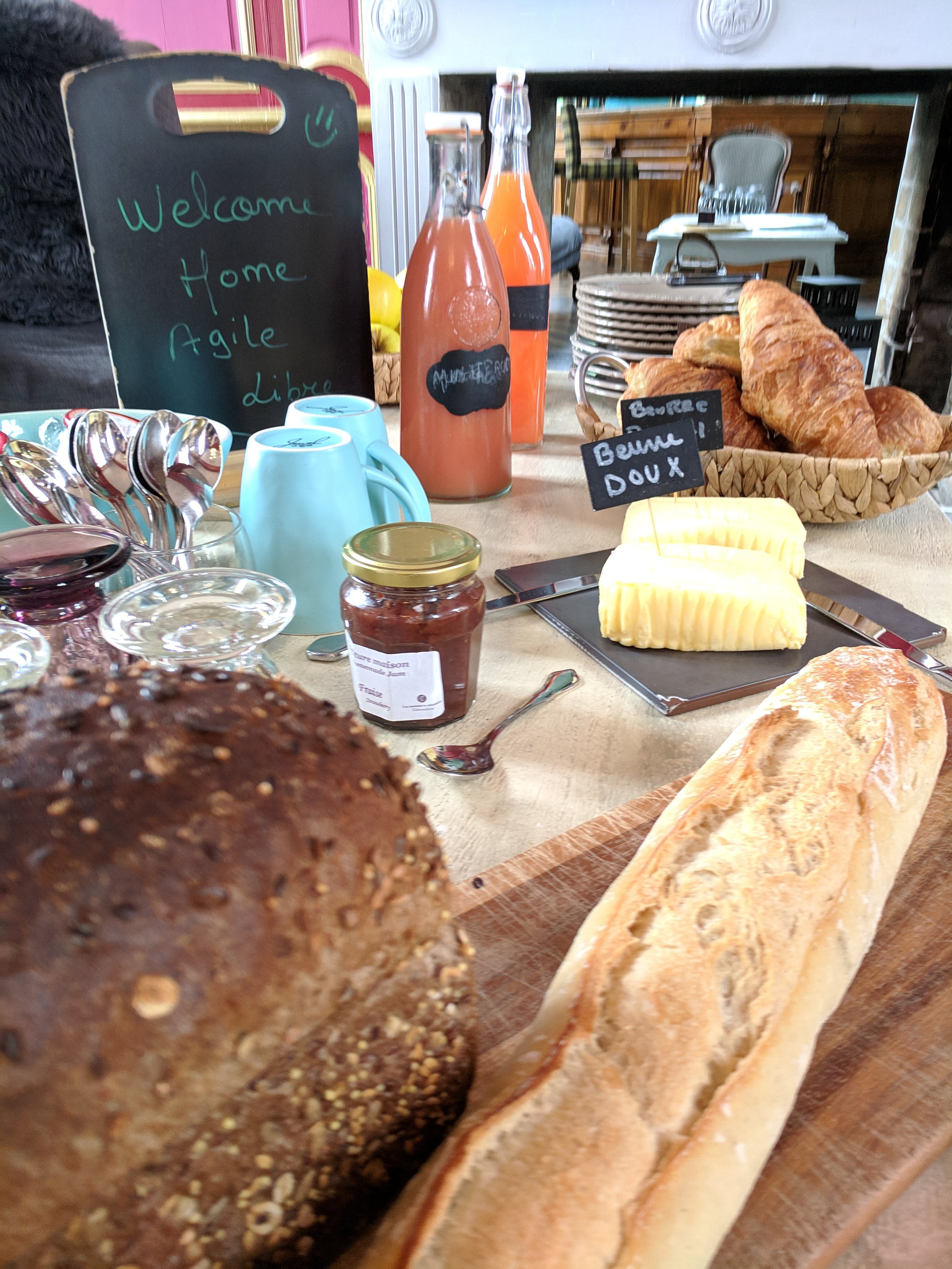
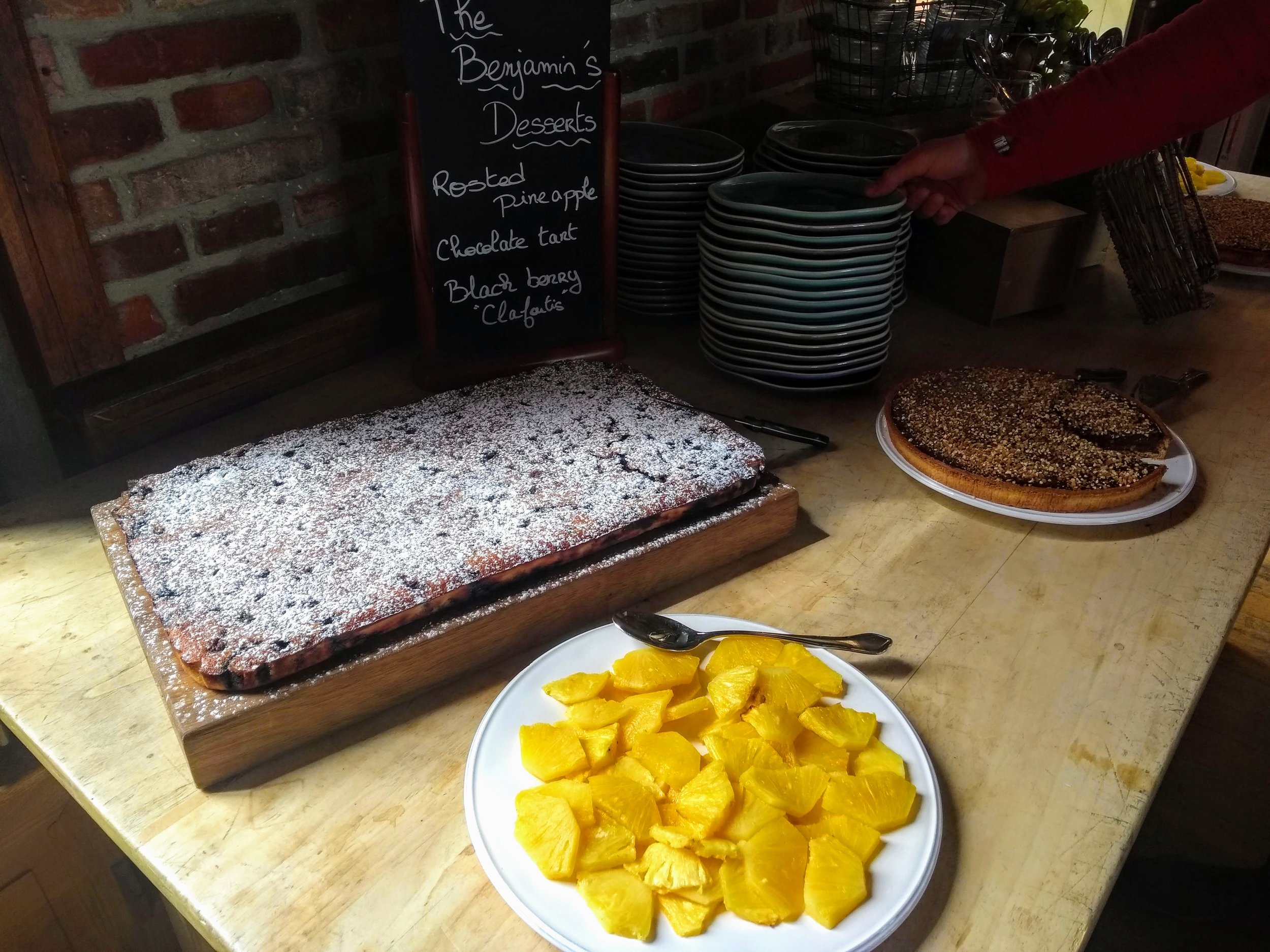
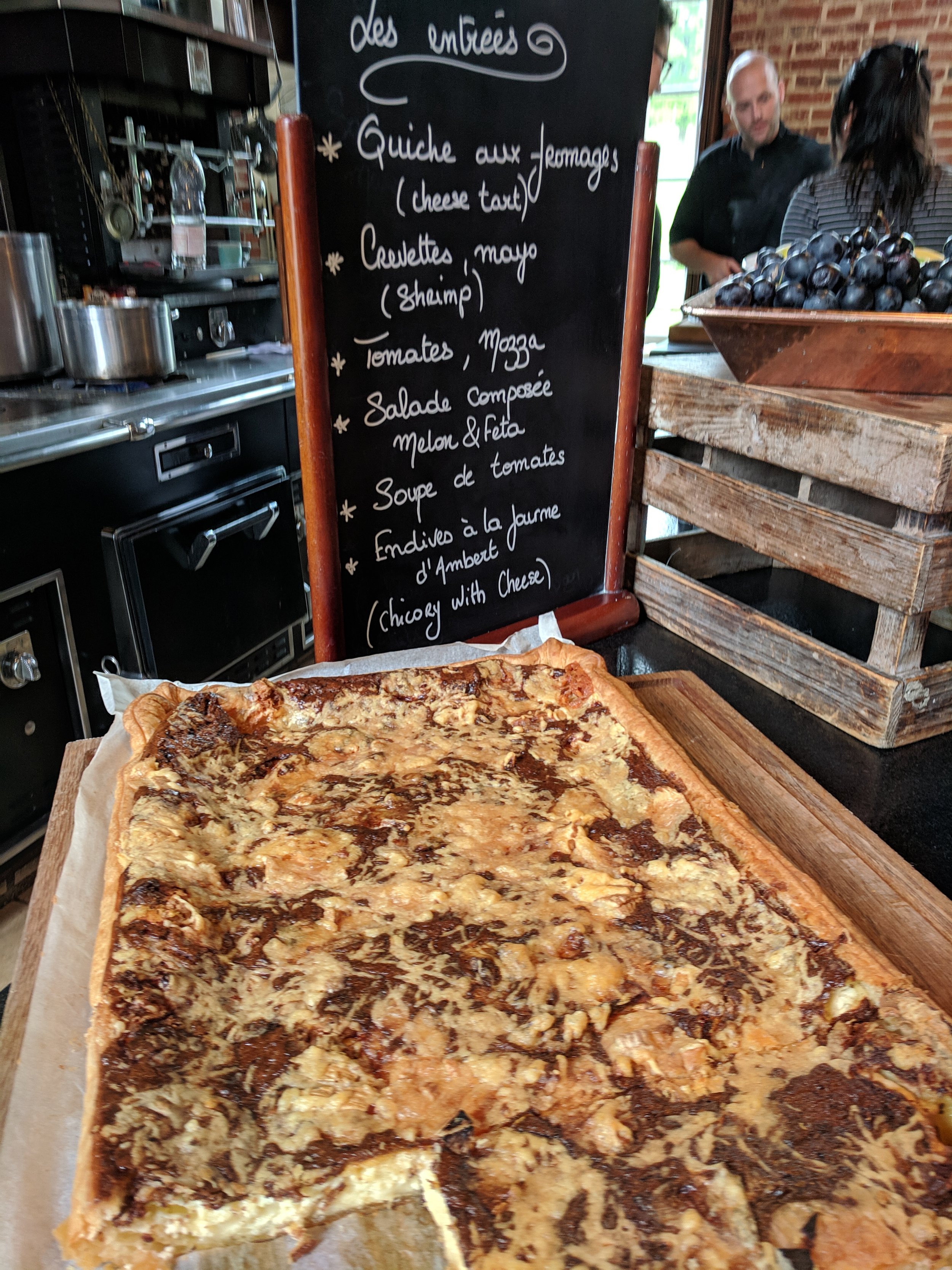
…but I’m not sure where to start. The full potential of food — to satisfy, to delight, to start conversations, to impress, to inspire — was realized. The food was central to the experience, but somehow not even the most wonderful thing about the experience of eating at the chateau. Meals were prefaced by a presentation by the professionals in the kitchen. No dish was repeated… indeed, no seating arrangement was repeated. The cheese was — if you are into cheese — off the charts.

There was a professionalism and thoughtfulness to the dining that can perhaps only be found in France.

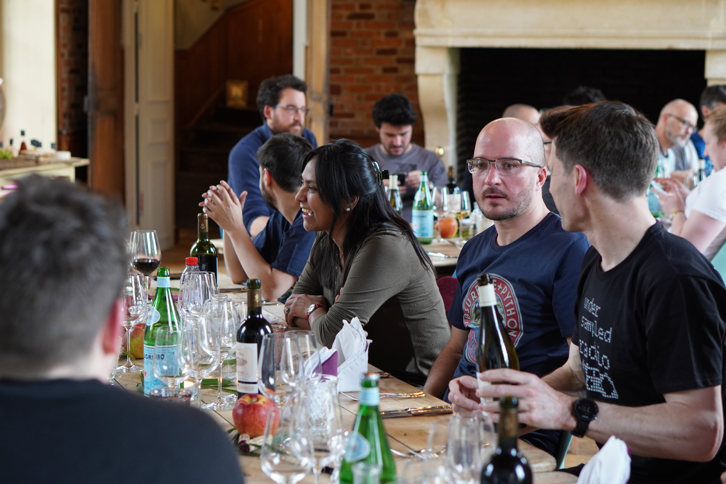
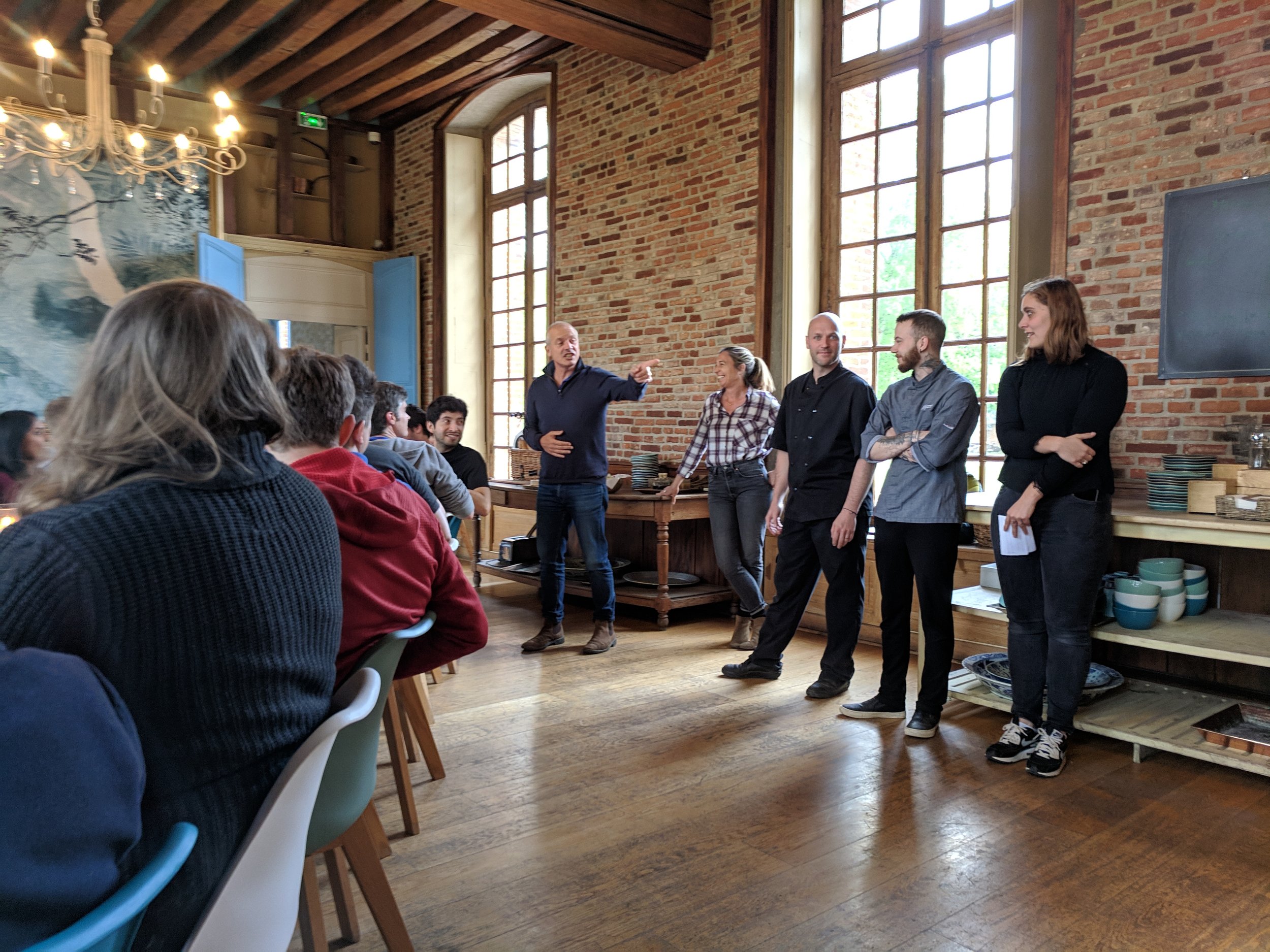
Sorry everyone. This was one of those occasions when you had to be there. If you weren’t there, you missed out. I wish you’d been there. You would have loved it.

The good news is that it will happen again. Stay tuned.

What's happening at TRANSFORM?

Last week, I laid out the case for naming and focusing on an open subsurface stack. To this end, we’re hosting TRANSFORM, an unconference, in May. At TRANSFORM, we’ll be mapping out the present state of things, imagining the future, and starting to build it together. You’re invited.

This week, I want to tell you a bit more about what’s happening at the unconference.

BYOS: Bring Your Own Session

We’ll be using an unconference model. If you come to the event, I ask you to prepare a 45 to 60 minute ‘slot’. You can do whatever you like in your slot, the only requirements are that it’s somewhat aligned with the theme (rocks, computers, and openness), and that it produces something tangible. For example:

• Start with a short presentation, maybe two, then hold a discussion. Capture the debate.

• Hold a brainstorming session, generating ideas for new technology. Record the ideas.

• Host a short sprint around a piece of existing software, checking code into GitHub.

• Research the available open tools for a particular workflow or file type. Report back.

Really, anything is possible. There’s no need to propose topics ahead of time (but please feel free to discuss them in the #transform channel on the Software Underground). We’ll be gathering all the topics and organizing the schedule for Monday, Tuesday and Wednesday on Sunday evening and Monday morning. It’s just-in-time conferencing!

After the unconference, then the sprints

By the end of Wednesday, we should have a very good idea of what’s in the open subsurface stack, and what is missing. On Thursday and Friday, we’ll have the opportunity to build things. In small team, we can take on all sorts of things:

• Improving the documentation of a project.

• Writing tutorials or course material for existing tools.

• Writing tests for an old or new project.

• Adding functionality to an old project, or even starting a new project.

By the end of Friday, we should have a big pile of new stuff to play with, and lots of new threads to follow after the event.

Here’s a first-draft, high-level view of the schedule so far…

The open subsurface stack

Two observations:

1. Agile has been writing about open source software for geology and geophysics for several years now (for example here in 2011 and here in 2016). Progress is slow. There are lots of useful tools, but lots of gaps too. Some new tools have appeared, others have died. Conclusion: a robust and trusted open stack is not going to magically appear.

2. People — some of them representing large corporations — are talking more than ever about industry collaboration. Open data platofrms are appearing all over the place. And several times at the DigEx conference in Oslo last week I heard people talk about open source and open APIs. Some organizations, notably Equinor, seem to really mean business. Conclusion: there seems to be a renewed appetite for open source subsurface software.

A quick reminder of what ‘open’ means; paraphrasing The Open Definition and The Open Source Definition in a sentence:

“Open data, content and code can be freely used, modified, and shared by anyone for any purpose.”

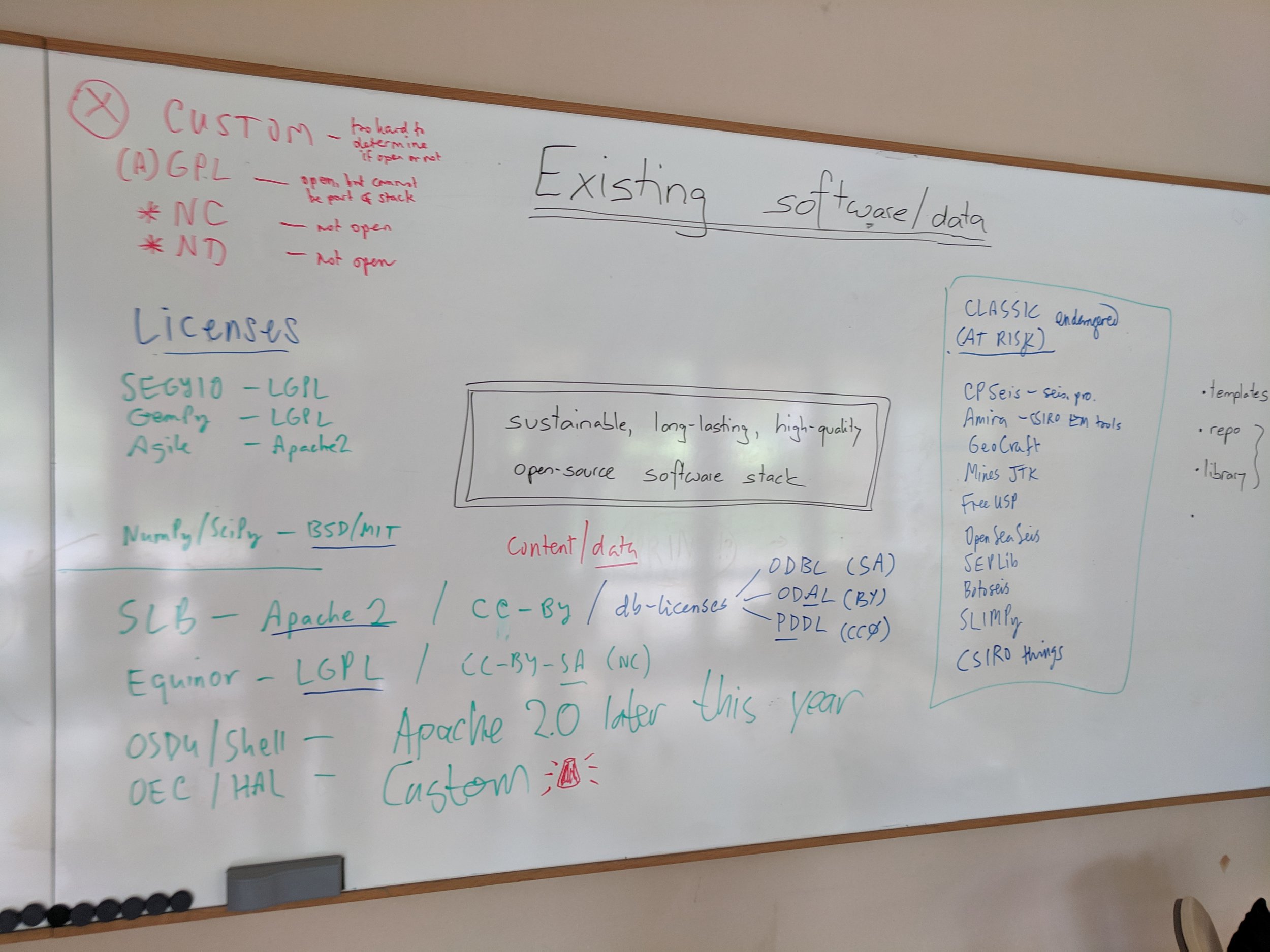
The word ‘open’ is being punted around quite a bit recently, but you have to read the small print in our business. Just as OpenWorks is not ‘open’ by the definition above, neither is OpenSpirit (remember that?), nor the Open Earth Community. (I’m not trying to pick on Halliburton but the company does seem drawn to the word, despite clearly not quite understanding it.)

The conditions are perfect

Earlier I said that a robust and trusted ‘stack’ (a collection of software that, ideally, does all the things we need) is not going to magically appear. What do I mean by ‘robust and trusted’? It goes far beyond ‘just code’ — writing code is the easy bit. It means thoroughly tested, carefully documented, supported, and maintained. All that stuff takes work, and work takes people and time. And people and time mean money.

Two more observations:

1. Agile has been teaching geocomputing like crazy — 377 people in the last year. In our class, the participants install a lot of Python libraries, including a few from the open subsurface stack: segyio, lasio, welly, and bruges. Conclusion: a proto-stack exists already, hundreds of users exist already, and some training and support exist already.

2. The Software Underground has over 1200 members (you should sign up, it’s free!). That’s a lot of people that care passionately about computers and rocks. The Python and machine learning communies are especially active. Conclusion: we have a community of talented scientists and developers that want to get good science done.

So what’s missing? What’s stopping us from taking open source subsurface tech to the next level?

Nothing!

Nothing is stopping us. And I’ve reached the conclusion that we need to provide care and feeding to this proto-stack, and this needs to start now. This is what the TRANSFORM 2019 unconference is going to be about. About 40 of us (you’re invited!) will spend five days working on some key questions:

• What libraries are in the Python ‘proto-stack’? What kind of licenses do they have? Who are the maintainers?

• Do we need a core library for the stack? Something to manage some basic data structures, units of measure, etc.

• What are we calling it, who cares about it, and how are we going to work together?

• Who has the capacity to provide attention, developer time, existing code, or funds to the stack?

• Where are the gaps in the stack, and which ones need to be filled first?

We won’t finish all this at the unconference. But we’ll get started. We’ll produce a lot of ideas, plans, roadmaps, GitHub issues, and new code. If that sounds like fun to you, and you can contribute something to this work — please come. We need you there! Get more info and sign up here.

---

Read the follow-up post >>> What’s happening at TRANSFORM?

---

Thumbnail photo of the Old Man of Hoy by Tom Bastin, CC-BY on Flickr.

What is the fastest axis of an array?

One of the participants in our geocomputing course asked us a tricky question earlier this year. She was a C++ and Java programmer — we often teach experienced programmers who want to learn about Python and/or machine learning — and she worked mostly with seismic data. She had a question related to the performance of n-dimensional arrays: what is the fastest axis of a NumPy array?

I’ve written before about how computational geoscience is not ‘software engineering’ and not ‘computer science’, but something else. And there’s a well established principle in programming, first expressed by Michael Jackson:

“We follow two rules in the matter of optimization:
Rule 1: Don’t do it.
Rule 2 (for experts only). Don’t do it yet — that is, not until you have a perfectly clear and unoptimized solution.”

Most of the time the computer is much faster than we need it to be, so we don’t spend too much time thinking about making our programs faster. We’re mostly concerned with making them work, then making them correct. But sometimes we have to think about speed. And sometimes that means writing smarter code. (Other times it means buying another GPU.) If your computer spends its days looping over seismic volumes extracting slices for processing, you should probably know whether you want to put time in the first dimension or the last dimension of your array.

The 2D case

Let’s think about a two-dimensional case first — imagine a small 2D array, also known as a matrix in some contexts. I’ve coloured in the elements of the matrix to make the next bit easier to understand.

When we store a matrix in a computer (or an image, or any array), we have a decision to make. In simple terms, the computer’s memory is like a long row of boxes, each with a unique address — shown here as a 3-digit hexadecimal number:

We can only store one number in each box, so we’re going to have to flatten the 2D array. The question is, do we put the rows in together, effectively splitting up the columns, or do we put the columns in together? These two options are commonly known as ‘row major’, or C-style, and ‘column major’, or Fortran-style:

Let’s see what this looks like in terms of the indices of the elements. We can plot the index number on each axis vs. the position of the element in memory. Notice that the C-ordered elements are contiguous in axis 0:

View fullsize

If you spend a lot of time loading seismic data, you probably recognize this issue — it’s analgous to how traces are stored in a SEG-Y file. Of couse, with seismic data, two dimensions aren’t always enough…

Higher dimensions

The problem multiplies at higher dimensions. If we have a cube of data, then C-style ordering results in the first dimension having large contiguous chunks, and the last dimension being broken up. The middle dimension is somewhere in between. As before, we can illustrating this by plotting the indices of the data. This time I’m highlighting the positions of the elements with index 2 (i.e. the third element) in each dimension:

So if this was a seismic volume, we might organize inlines in the first dimension, and travel-time in the last dimension. That way, we can access inlines very quickly, but timeslices will take longer.

In Fortran order, which we can optionally specify in NumPy, the situation is reversed. Now the fast axis is the last axis:

Lots of programming languages and libraries use row-major memory layout, including C, C++, Torch and NumPy. Most others use column-major ordering, including MATLAB, R, Julia, and Fortran. (Some other languages, such as Java and .NET, use a variant of row-major order called Iliffe vectors). NumPy calls row-major order ‘C’ (for C, not for column), and column-major ‘F’ for Fortran (thankfully they didn’t use R, for R not for row).

I expect it’s related to their heritage, but the Fortran-style languages also start counting at 1, whereas the C-style languages, including Python, start at 0.

What difference does it make?

The main practical difference is in the time it takes to access elements in different orientations. It’s faster for the computer to take a contiguous chunk of neighbours from the memory ‘boxes’ than it is to have to ‘stride’ across the memory taking elements from here and there.

How much faster? To find out, I made datasets full of random numbers, then selected slices and added 1 to them. This was the simplest operation I could think of that actually forces NumPy to do something with the data. Here are some statistics — the absolute times are pretty irrelevant as the data volumes I used are all different sizes, and the speeds will vary on different machines and architectures:

• 2D data: 3.6× faster. Axis 0: 24.4 µs, axis 1: 88.1 µs (times relative to first axis: 1, 3.6).

• 3D data: 43× faster. 229 µs, 714 µs, 9750 µs (relatively 1, 3.1, 43).

• 4D data: 24× faster. 1.27 ms, 1.36 ms, 4.77 ms, 30 ms (relatively 1, 1.07, 3.75, 23.6).

• 5D data: 20× faster. 3.02 ms, 3.07 ms, 5.42 ms, 11.1 ms, 61.3 ms (relatively 1, 1.02, 1.79, 3.67, 20.3).

• 6D data: 5.5× faster. 24.4 ms, 23.9 ms, 24.1 ms, 37.8 ms, 55.3 ms, 136 ms (relatively 1, 0.98, 0.99, 1.55, 2.27, 5.57).

These figures are more or less simply reversed for Fortran-ordered arrays (see the notebook for datails).

Clearly, the biggest difference is with 3D data, so if you are manipulating seismic data a lot and need to access the data in that last dimension, usually travel-time, you might want to think about ways to reduce this overhead.

What difference does it really make?

The good news is that, for most of us most of the time, we don’t have to worry about any of this. For one thing, NumPy’s internal workings (in particular, its universal functions, or ufuncs) know which directions are fastest and take advantage of this when possible. For another thing, we generally try to avoid looping over arrays at all, leaving the iterative components of our algorithms to the ufuncs — so the slicing speed isn’t a factor. Even when it is a factor, or if we can’t avoid looping, it’s often not the bottleneck in the code. Usually the guts of our algorithm are what are slowing the computer down, not the access to memory. The net result of all this is that we don’t often have to think about the memory layout of our arrays.

So when does it matter? The following situations merit a bit of thought:

• When you’re doing a very large number of accesses to memory or disk. Saving a few microseconds might add up to a lot if you’re doing it a billion times.

• When the objects you’re accessing are very large. Reading and writing elements of a 200GB array in memory brings new challenges compared to handling a few gigabytes.

• Reading and writing data files — really just another kind of memory — brings all the same issues. Reading a chunk of contiguous data is much faster than reading bytes from here and there. Landmark’s BRI seismic data format, Schlumberger’s ZGY files, and HDF5 files, all implement strategies to help make reading arbitrary data faster.

• Converting code from other languages, especially MATLAB, although do realize that other languages may have their own indexing rules, as well as differing in how they store n-dimensional arrays.

If you determine that you do need to think about this stuff, then you’re going to need to read this essay about NumPy’s internal representations, and I recommend checking out this blog post by Eli Bendersky too.

There you have it. Very occasionally we scientists also need to think a bit about how computers work… but most of the time someone has done that thinking for us.

Some of the figures and all of the timings for this post came from this notebook — please have a look. If you have anything to add, or (better yet) correct, please get in touch. I’d love to hear from you.

TRANSFORM 2019

Yesterday I announced that we’re hatching a new plan. The next thing. Today I want to tell you about it.

The project has the codename TRANSFORM. I like the notion of transforms: functions that move you from one domain to another. Fourier transforms. Wavelet transforms. Digital subsurface transforms. Examples:

• The transformative effect of open source software on subsurface science. Open source accelerates our work!

• The transformative effect of collaborative, participatory events on the community. We can make new things!

• The transformative effect of training on ourselves and our peers. Lots of us have new superpowers!

Together, we’ve built the foundation for a new, open software platform.

A domain shift

We think it’s time to refocus the hackathons as sprints — purposefully producing a sustainable, long-lasting, high quality, open source software stack that we can all use and combine into new tools, whether open or proprietary, free or commercial.

We think it’s time to bring a full-featured unconference into the mix. The half-day ‘unsessions’ open too many paths, and leave too few explored. We need more time — to share research, plan software projects, and write code.

Together, we can launch a new era in scientific computing for the subsurface.

At the core of this new era core is a new open-source software stack, created, maintained, and implemented by a community of scientists and organizations passionate about its potential.

Sign up!

Here’s the plan. We’re hosting an unconference from 5 to 11 May 2019, with full days from Monday to Friday. The event will take place at the Château de Rosay, near Rouen, France. It will be fully residential and fully catered. We have room for about 45 participants.

The goal is to lay down a road map for designing, funding, and building an open source software stack for subsurface. In the coming days and weeks, we will formulate the plan for the week, with input from the Software Underground. We want to hear from you. Propose a session! Host a sprint! Offer a bounty! There are lots of ways to get involved.

View fullsize

Map data: GeoBasis-DE / BKG / Google, photo: Chateauform. Click to enlarge.

If you want to be part of this effort, as a developer, an end-user, or a sponsor, then we invite you to join us.

The unconference fee will be EUR 1000, and accommodation and food will be EUR 1500. The student fees will be EUR 240 and EUR 360. There will be at least 5 bursaries of EUR 1000 available.

For the time being, we will be accepting early commitments, with a deposit of EUR 400 to secure a place (students wishing to register now should get in touch). Soon, you will be able to sign up online… we are working on a smooth process. In the meantime, click here to register your interest, share ideas for content, or sign up by paying a deposit.

Thanks for reading. We look forward to figuring this out together.

---

I’m delighted to be able to announce that we already have support from Dell EMC. Thanks as ever to David Holmes for his willingness to fund experiments!

---

In the US or Canada? Don’t despair! There will be a North American edition in Quebec in late September.

The next thing

Over the last several years, Agile has been testing some of the new ways of collaborating, centered on digital connections:

• It all started with this blog, which started in 2010 with my move from Calgary to Nova Scotia. It’s become a central part of my professional life, but we’re all about collaboration and blogs are almost entirely one-way, so…

• In 2011 we launched SubSurfWiki. It didn’t really catch on, although it was a good basis for some other experiments and I still use it sometimes. Still, we realized we had to do more to connect the community, so…

• In 2012 we launched our 52 Things collaborative, open access book series. There are well over 5000 of these out in the wild now, but it made us crave a real-life, face-to-face collaboration, so…

• In 2013 we held the first ‘unsession’, a mini-unconference, at the Canada GeoConvention. Over 50 people came to chat about unsolved problems. We realized we needed a way to actually work on problems, so…

• Later that year, we followed up with the first geoscience hackathon. Around 15 or so of us gathered in Houston for a weekend of coding and tacos. We realized that the community needed more coding skills, so…

• In 2014 we started teaching a one-day Python course aimed squarely at geoscientists. We only teach with subsurface data and algorithms, and the course is now 5 days long. We now needed a way to connect all these new hackers and coders, so…

• In 2014, together with Duncan Child, we also launched Software Underground, a chat room for discussing topics related to the earth and computers. Initially it was a Google Group but in 2015 we relaunched it as an open Slack team. We wanted to double down on scientific computing, so…

• In 2015 and 2016 we launched a new web app, Pick This (returning soon!), and grew our bruges and welly open source Python projects. We also started building more machine learning projects, and getting really good at it.

Growing and honing

We have spent the recent years growing and honing these projects. The blog gets about 10,000 readers a month. The sixth 52 Things book is on its way. We held two public unsessions this year. The hackathons have now grown to 60 or so hackers, and have had about 400 participants in total, and five of them this year already (plus three to come!). We have also taught Python to 400 geoscientists, including 250 this year alone. And the Software Underground has over 1000 members.

In short, geoscience has gone digital, and we at Agile are grateful and excited to be part of it. At no point in my career have I been more optimistic and energized than I am right now.

So it’s time for the next thing.

The next thing is starting with a new kind of event. The first one is 5 to 11 May 2019, and it’s happening in France. I’ll tell you all about it tomorrow.

Reproducibility Zoo

The Repro Zoo was a new kind of event at the SEG Annual Meeting this year. The goal: to reproduce the results from well-known or important papers in GEOPHYSICS or The Leading Edge. By reproduce, we meant that the code and data should be open and accessible. By results, we meant equations, figures, and other scientific outcomes.

And some of the results are scary enough for Hallowe’en :)

What we did

All the work went straight into GitHub, mostly as Jupyter Notebooks. I had a vague goal of hitting 10 papers at the event, and we achieved this (just!). I’ve since added a couple of other papers, since the inspiration for the work came from the Zoo… and I haven’t been able to resist continuing.

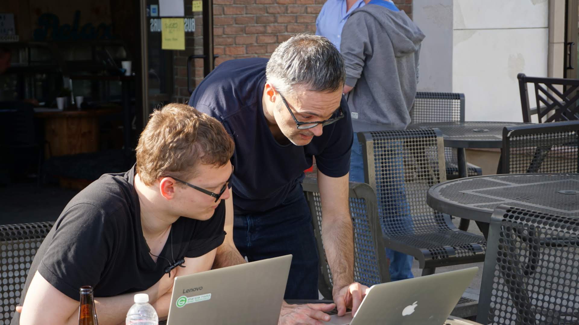
The scene at the Repro Zoo. An air of quiet productivity hung over the booth. Yes, that is Sergey Fomel and Jon Claerbout. Thank you to David Holmes of Dell EMC for the picture.

Here’s what the Repro Zoo team got up to, in alphabetical order:

• Aldridge (1990). The Berlage wavelet. GEOPHYSICS 55 (11). The wavelet itself, which has also been added to bruges.

• Batzle & Wang (1992). Seismic properties of pore fluids. GEOPHYSICS 57 (11). The water properties, now added to bruges.

• Claerbout et al. (2018). Data fitting with nonstationary statistics, Stanford. Translating code from FORTRAN to Python.

• Claerbout (1975). Kolmogoroff spectral factorization. Thanks to Stewart Levin for this one.

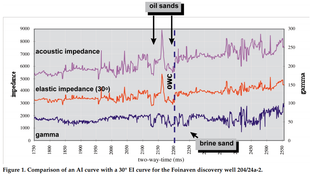
• Connolly (1999). Elastic impedance. The Leading Edge 18 (4). Using equations from bruges to reproduce figures.

• Liner (2014). Long-wave elastic attentuation produced by horizontal layering. The Leading Edge 33 (6). This is the stuff about Backus averaging and negative Q.

• Luo et al. (2002). Edge preserving smoothing and applications. The Leading Edge 21 (2).

• Yilmaz (1987). Seismic data analysis, SEG. Okay, not the whole thing, but Sergey Fomel coded up a figure in Madagascar.

• Partyka et al. (1999). Interpretational aspects of spectral decomposition in reservoir characterization.

• Röth & Tarantola (1994). Neural networks and inversion of seismic data. Kudos to Brendon Hall for this implementation of a shallow neural net.

• Taner et al. (1979). Complex trace analysis. GEOPHYSICS 44. Sarah Greer worked on this one.

• Thomsen (1986). Weak elastic anisotropy. GEOPHYSICS 51 (10). Reproducing figures, again using equations from bruges.

As an example of what we got up to, here’s Figure 14 from Batzle & Wang’s landmark 1992 paper on the seismic properties of pore fluids. My version (middle, and in red on the right) is slightly different from that of Batzle and Wang. They don’t give a numerical example in their paper, so it’s hard to know where the error is. Of course, my first assumption is that it’s my error, but this is the problem with research that does not include code or reference numerical examples.

View fullsize

Figure 14 from Batzle & Wang (1992). Left: the original figure. Middle: My attempt to reproduce it. Right: My attempt in red, overlain on the original.

This was certainly not the only discrepancy. Most papers don’t provide the code or data to reproduce their figures, and this is a well-known problem that the SEG is starting to address. But most also don’t provide worked examples, so the reader is left to guess the parameters that were used, or to eyeball results from a figure. Are we really OK with assuming the results from all the thousands of papers in GEOPHYSICS and The Leading Edge are correct? There’s a long conversation to have here.

What next?

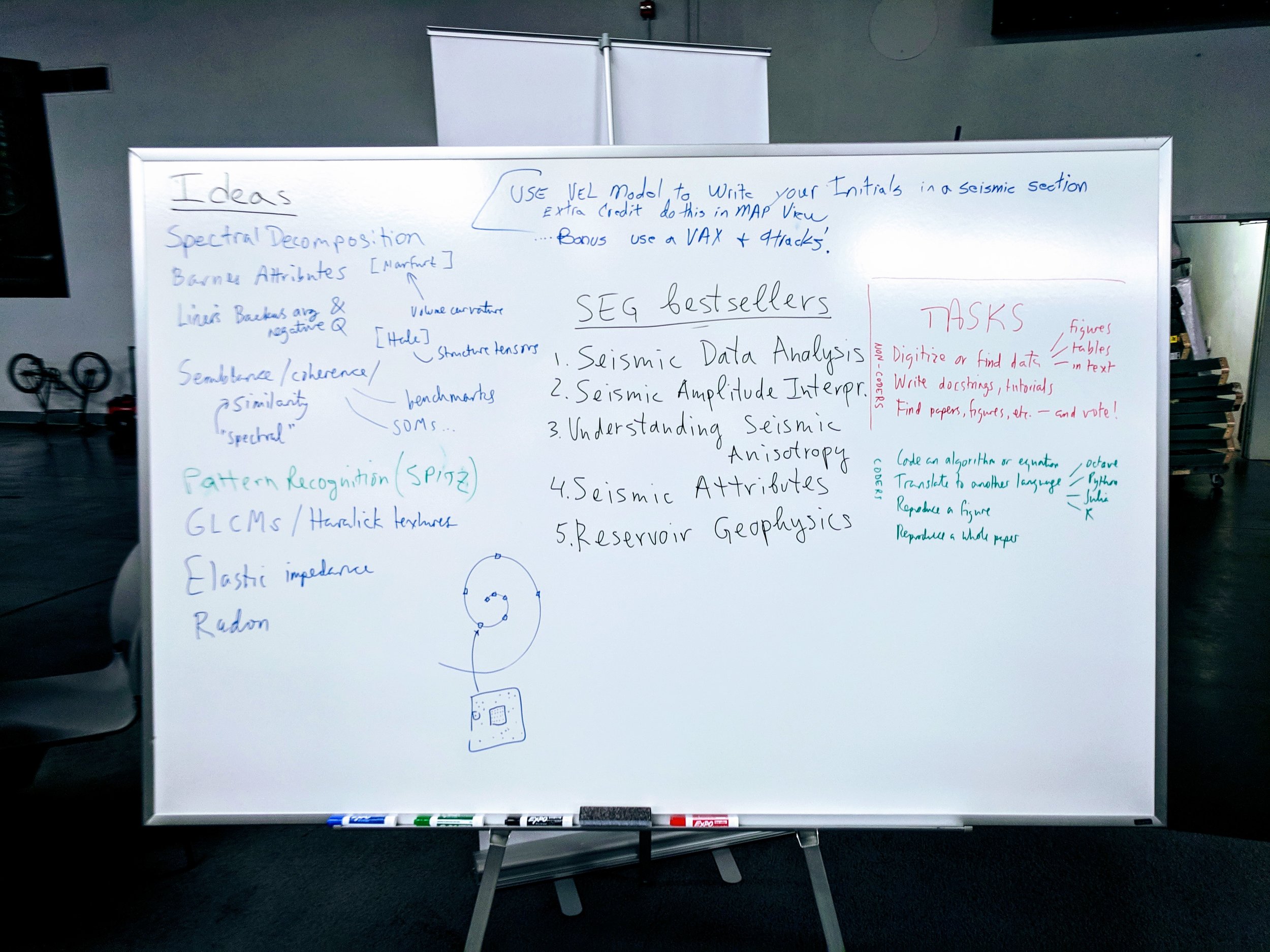
One thing we struggled with was capturing all the ideas. Some are on our events portal. The GitHub repo also points to some other sources of ideas. And there was the Big Giant Whiteboard (below). Either way, there’s plenty to do (there are thousands of papers!) and I hope the zoo continues in spirit. I will take pull requests until the end of the year, and I don’t see why we can’t add more papers until then. At that point, we can start a 2019 repo, or move the project to the SEG Wiki, or consider our other options. Ideas welcome!

Thank you!

The following people and organizations deserve accolades for their dedication to the idea and hard work making it a reality. Please give them a hug or a high five when you see them.

• David Holmes (Dell EMC) and Chance Sanger worked their tails off on the booth over the weekend, as well as having the neighbouring Dell EMC booth to worry about. David also sourced the amazing Dell tech we had at the booth, just in case anyone needed 128GB of RAM and an NVIDIA P5200 graphics card for their Jupyter Notebook. (The lights in the convention centre actually dimmed when we powered up our booths in the morning.)

• Luke Decker (UT Austin) organized a corps of volunteer Zookeepers to help manage the booth, and provided enthusiasm and coding skills. Karl Schleicher (UT Austin), Sarah Greer (MIT), and several others were part of this effort.

• Andrew Geary (SEG) for keeping things moving along when I became delinquent over the summer. Lots of others at SEG also helped, mainly with the booth: Trisha DeLozier, Rebecca Hayes, and Beth Donica all contributed.

• Diego Castañeda got the events site in shape to support the Repro Zoo, with a dashboard showing the latest commits and contributors.

Café con leche

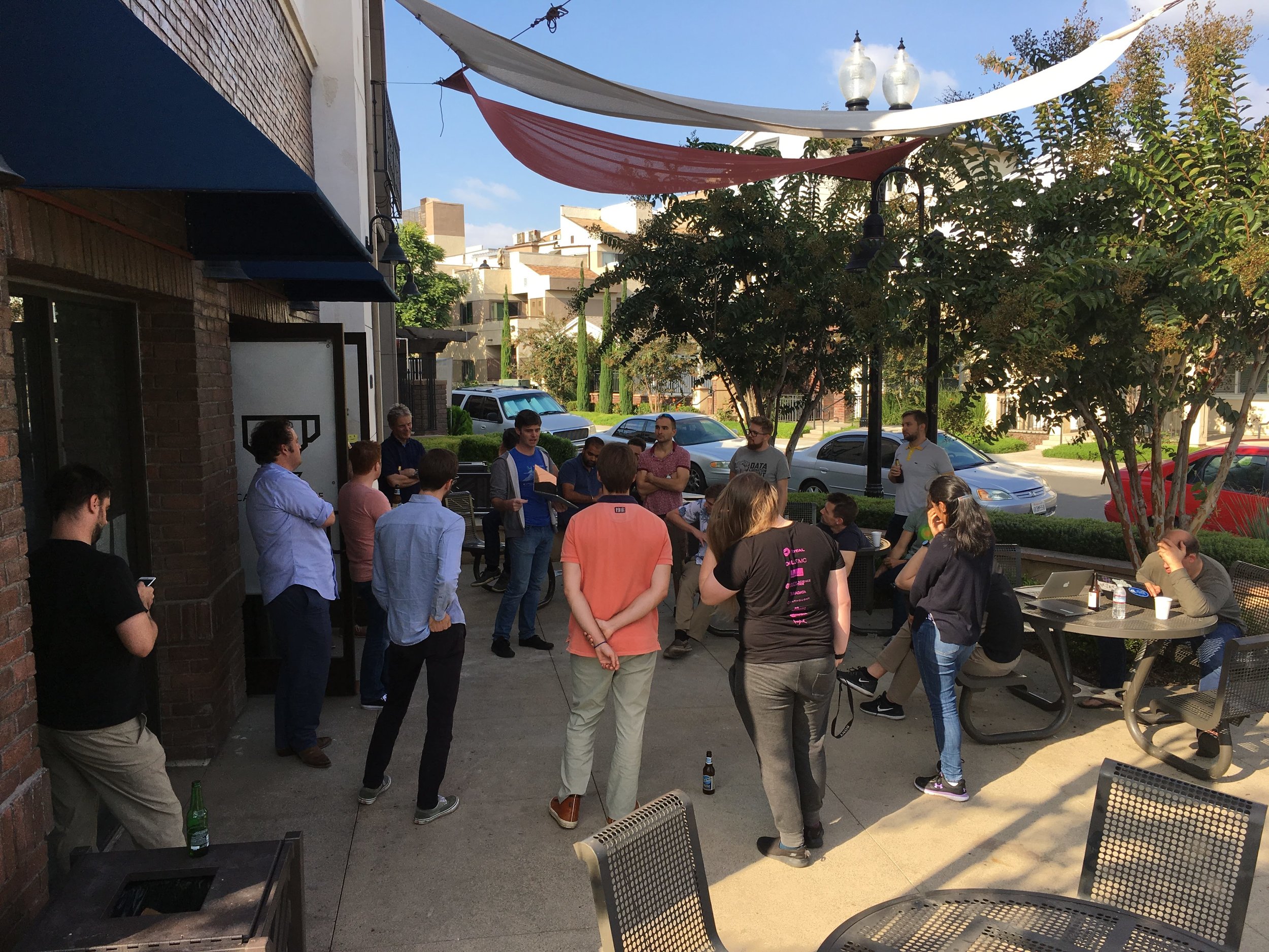
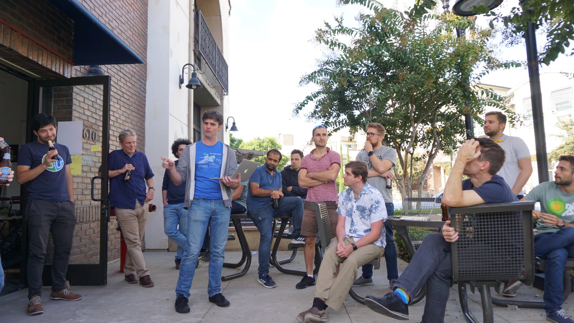
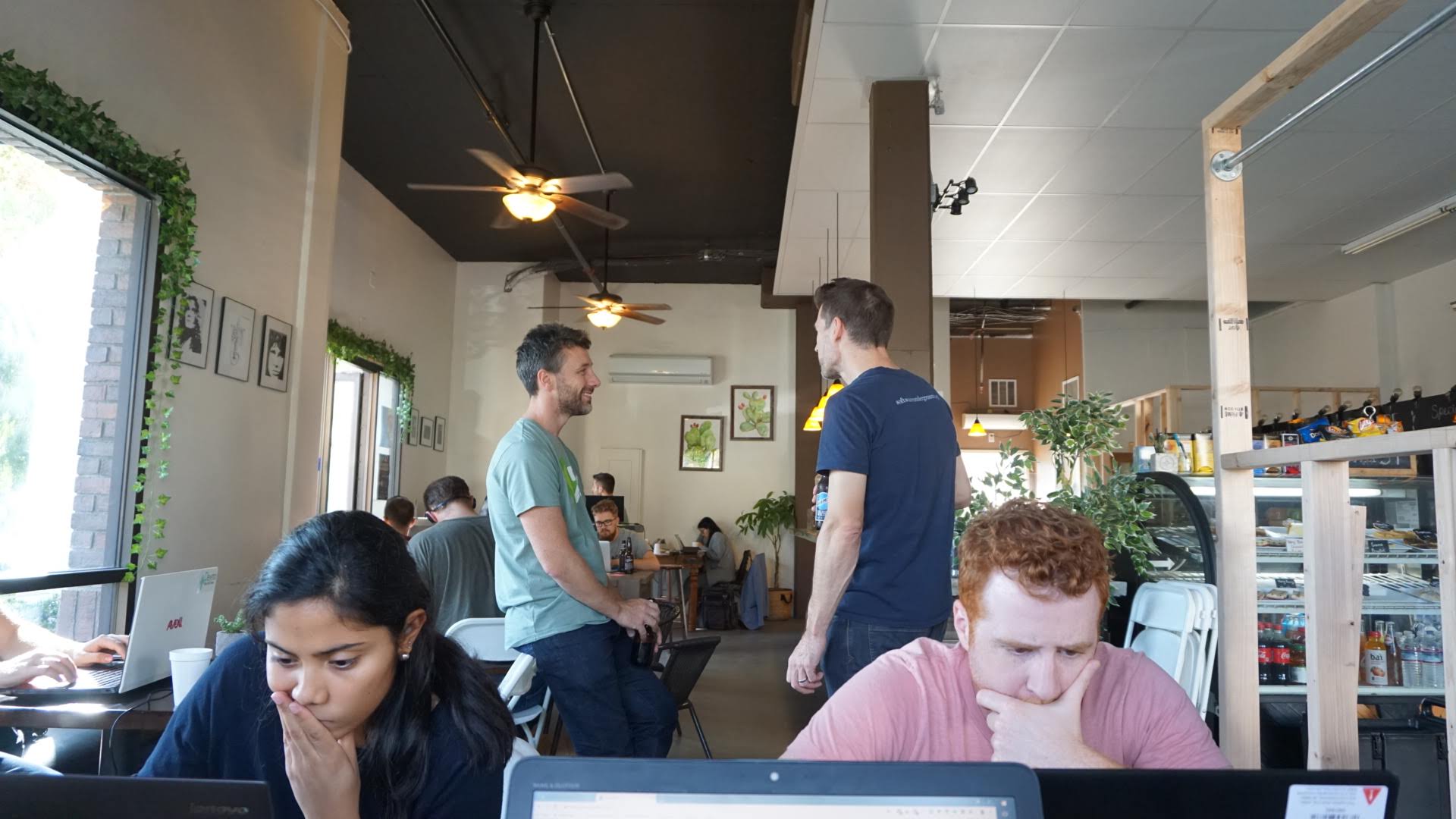
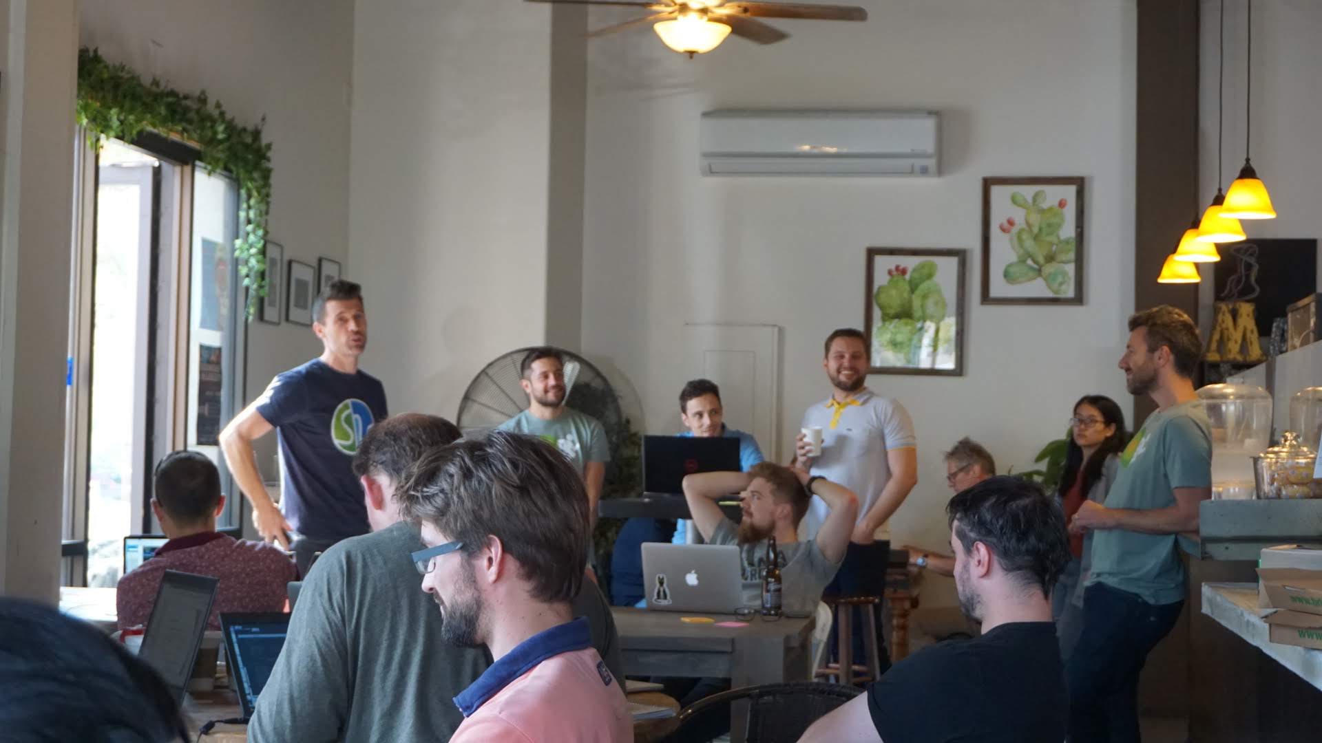
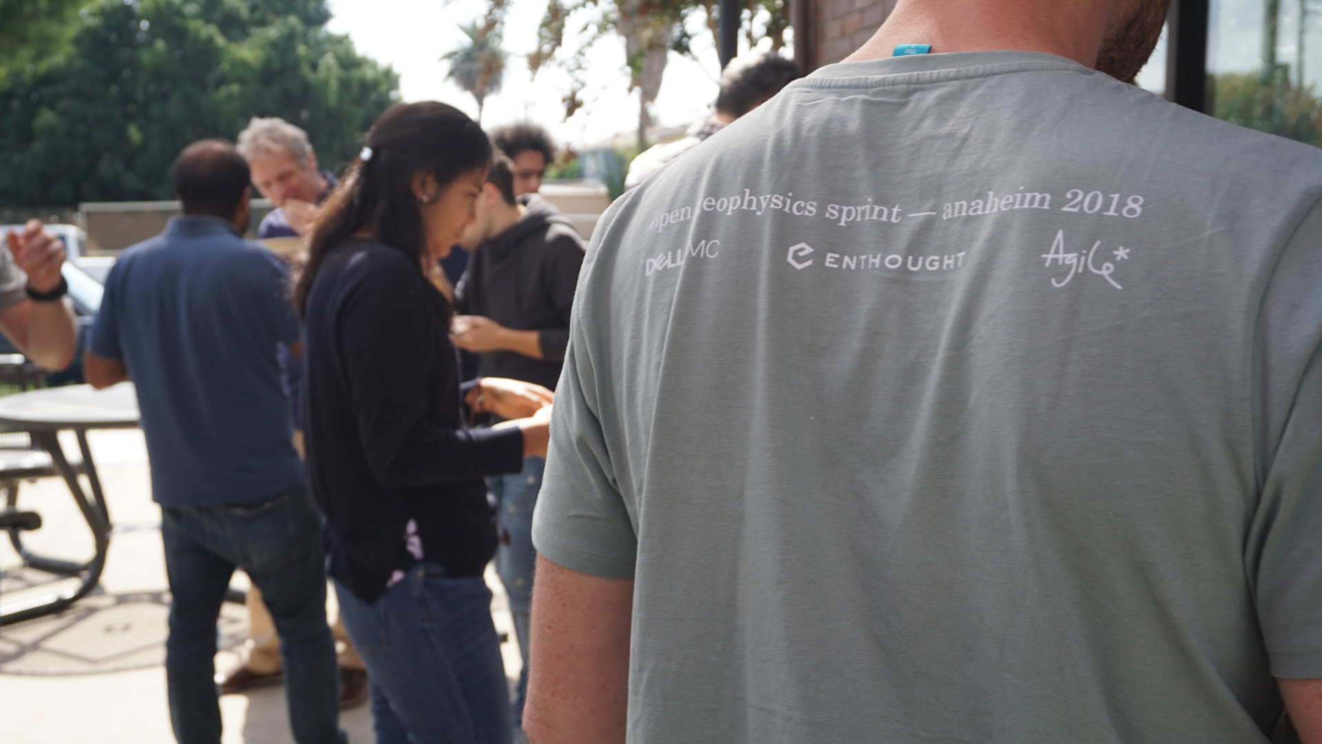
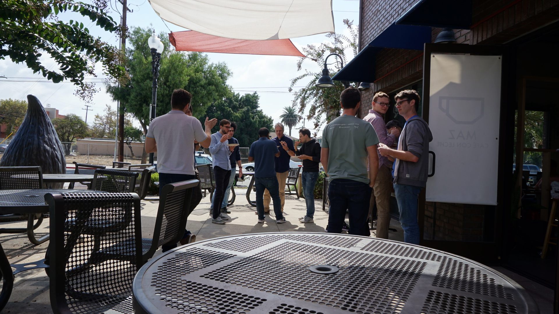
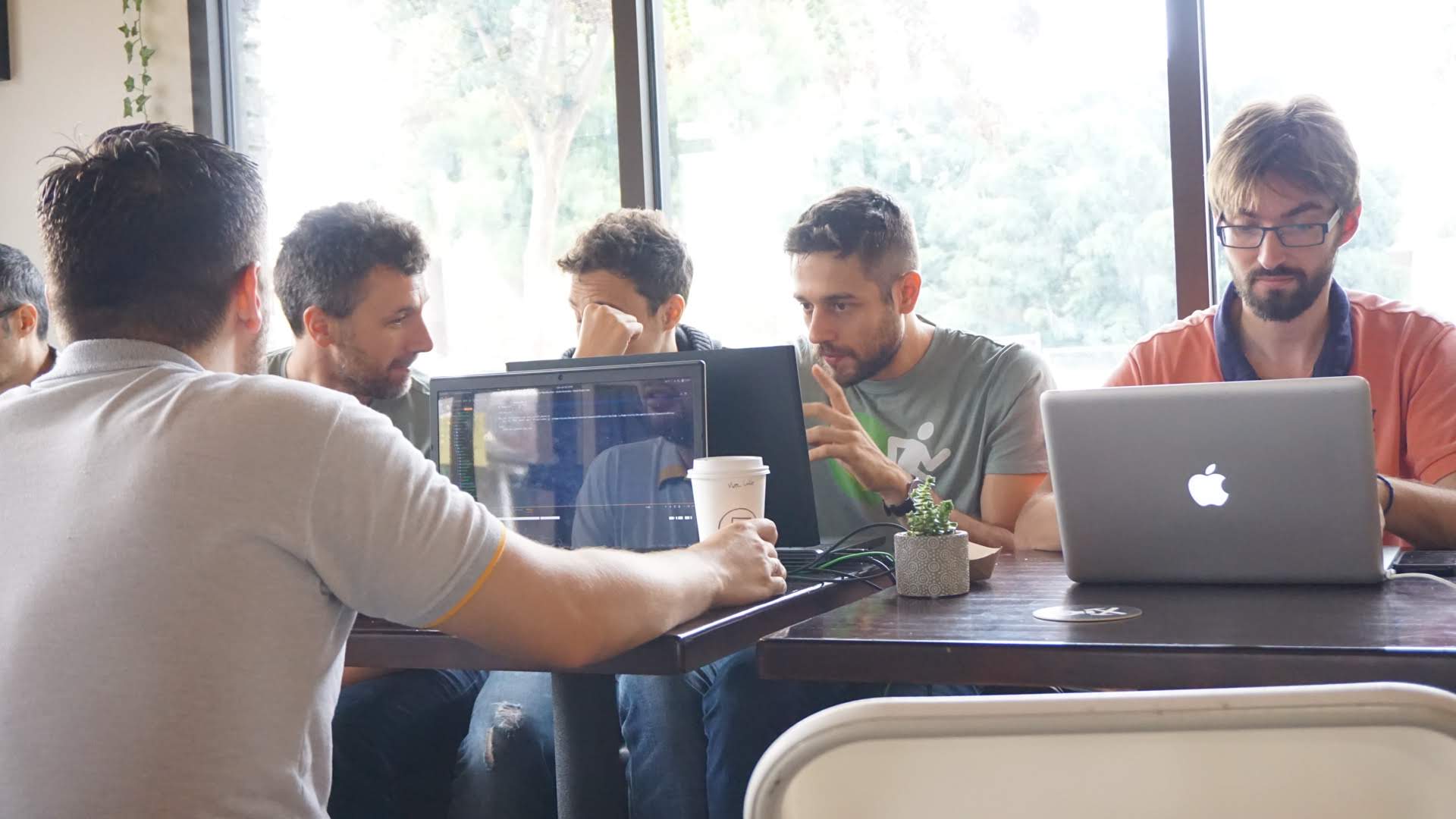
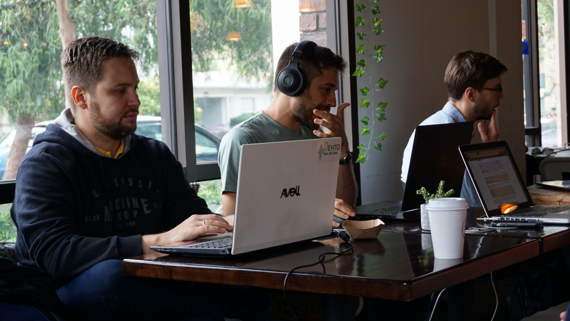
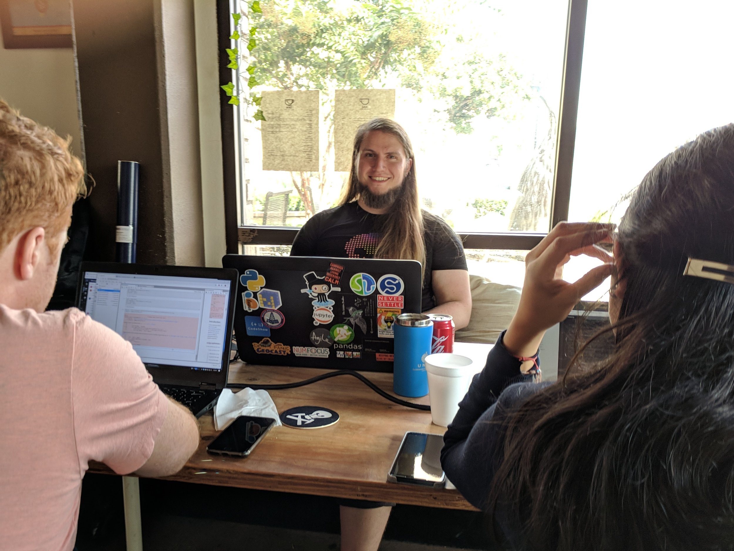
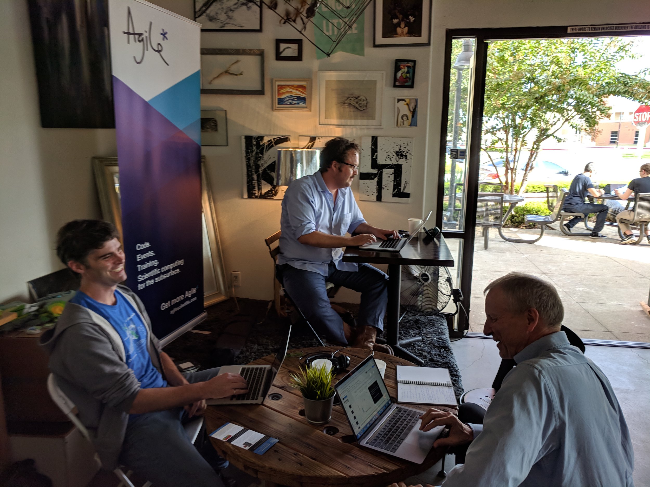
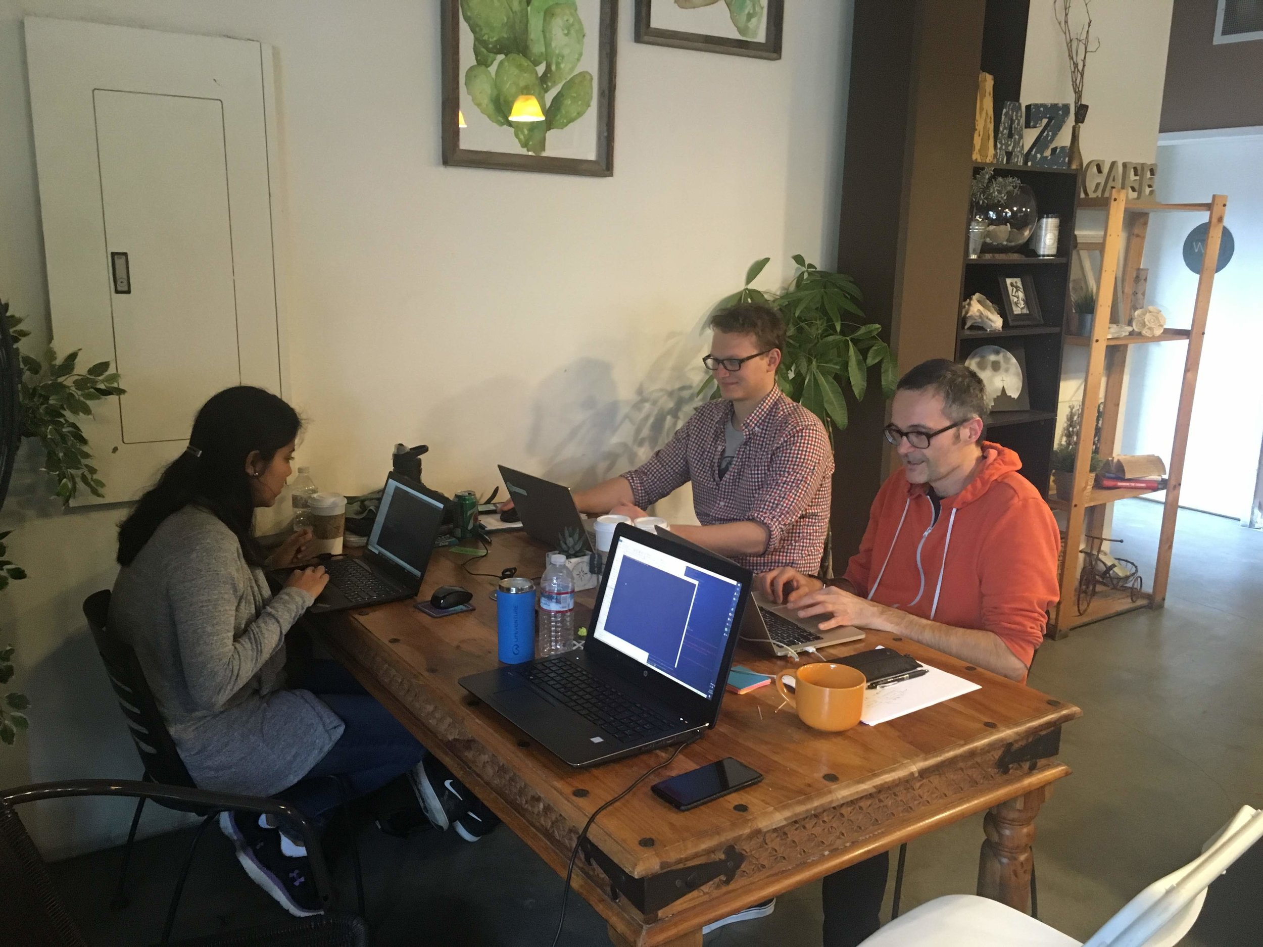
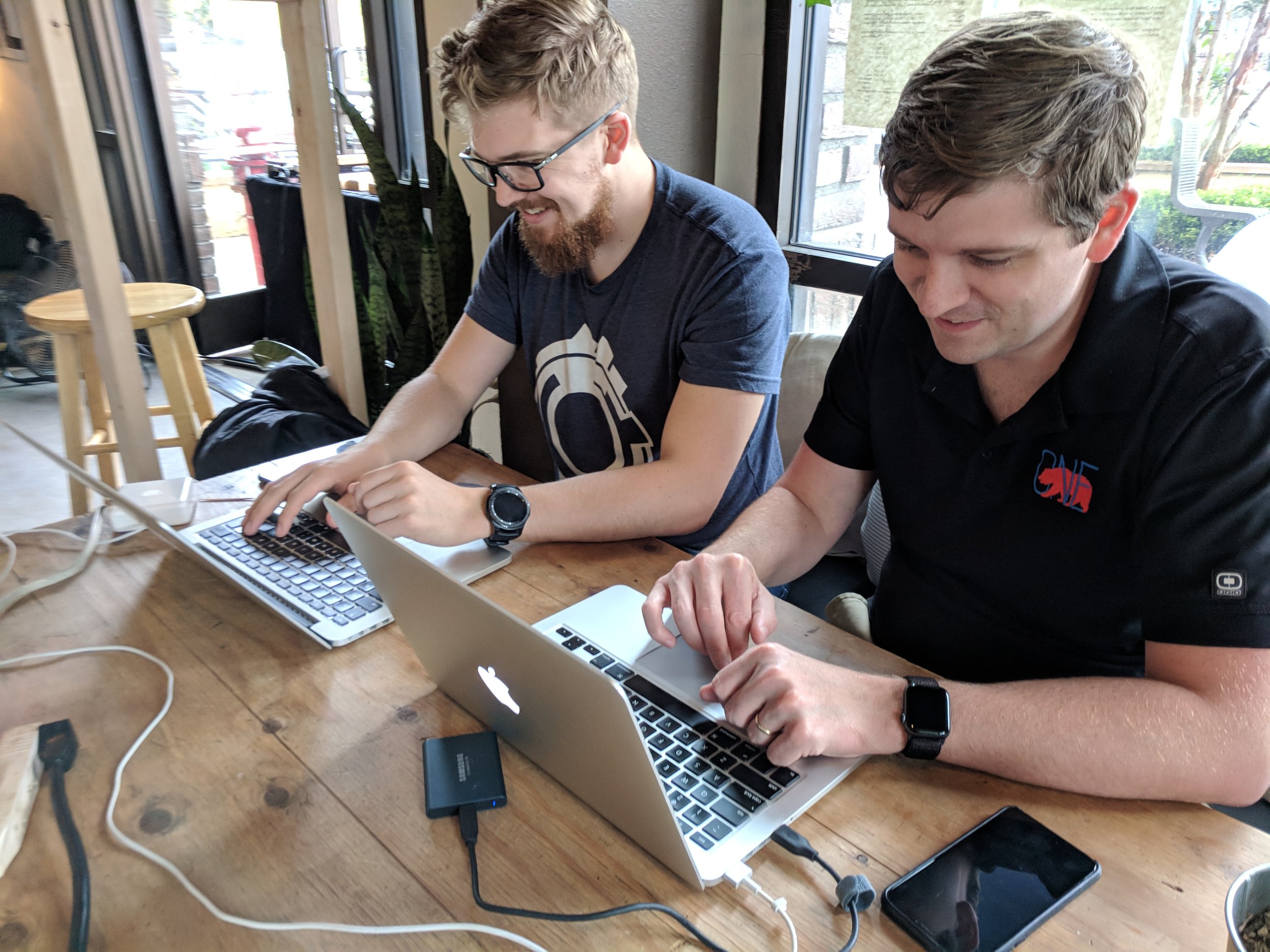
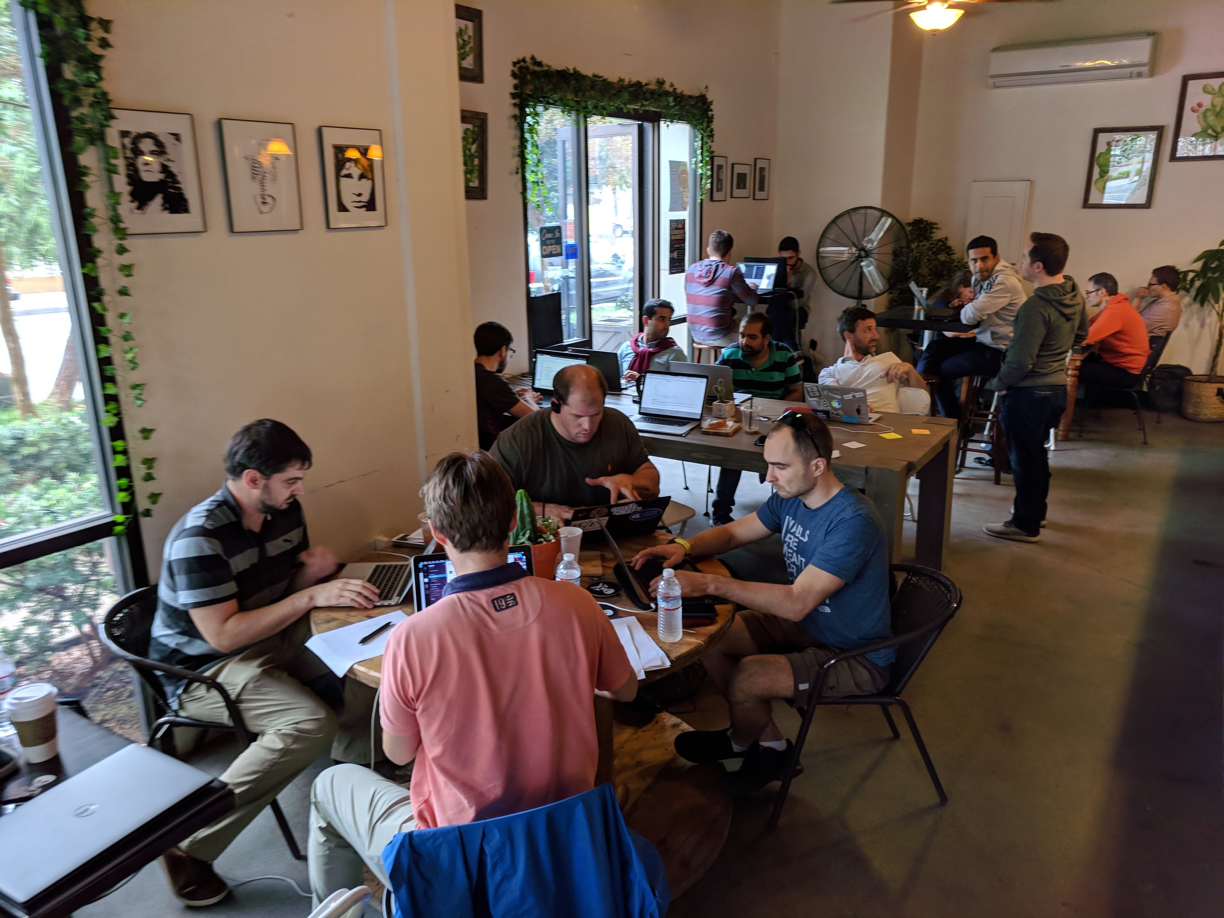
At the weekend, 28 digital geoscientists gathered at MAZ Café in Santa Ana, California, to sprint on some open geophysics software projects. Teams and individuals pushed pull requests — code contributions to open source projects — left, right, and centre. Meanwhile, Senah and her team at MAZ kept us plied with coffee and horchata, with fantastic food on the side.

View fullsize

Because people were helping each other and contributing where they could, I found it a bit hard to stay on top of what everyone was working on. But here are some of the things I heard at the project breakdown on Sunday afternoon:

Gerard Gorman, Navjot Kukreja, Fabio Luporini, Mathias Louboutin, and Philipp Witte, all from the devito project, continued their work to bring Kubernetes cluster management to devito. Trying to balance ease of use and unlimited compute turns out to be A Hard Problem! They also supported the other teams hacking on devito.

Thibaut Astic (UBC) worked on implementing DC resistivity models in devito. He said he enjoyed the expressiveness of devito’s symbolic equation definitions, but that there were some challenges with implementing the grad, div, and curl operator matrices for EM.

Vitor Mickus and Lucas Cavalcante (Campinas) continued their work implementing a CUDA framework for devito. Again, all part of the devito project trying to give scientists easy ways to scale to production-scale datasets.

That wasn’t all for devito. Alongside all these projects, Stephen Alwon worked on adapting segyio to read shot records, Robert Walker worked on poro-elastic models for devito, and Mohammed Yadecuri and Justin Clark (California Resources) contributed too. On the second day, the devito team was joined by Felix Hermann (now Georgia Tech), with Mengmeng Yang, and Ali Siakoohi (both UBC). Clearly there’s something to this technology!

Brendon Hall and Ben Lasscock (Enthought) hacked on an open data portal concept, based on the UCI Machine Learning Repository, coincidentally based just down the road from our location. The team successfully got some examples of open data and code snippets working.

Jesper Dramsch (Heriot-Watt), Matteo Niccoli (MyCarta), Yuriy Ivanov (NTNU) and Adriana Gordon and Volodymyr Vragov (U Calgary), hacked on bruges for the weekend, mostly on its documentation and the example notebooks in the in-bruges project. Yuriy got started on a ray-tracing code for us.

Nathan Jones (California Resources) and Vegard Hagen (NTNU) did some great hacking on an interactive plotting framework for geoscience data, based on Altair. What they did looked really polished and will definitely come in useful at future hackathons.

All in all, an amazing array of projects!

This event was low-key compared to recent hackathons, and I enjoyed the slightly more relaxed atmosphere. The venue was also incredibly supportive, making my life very easy.

A big thank you as always to our sponsors, Dell EMC and Enthought. The presence of the irrepressible David Holmes and Chris Lenzsch (both Dell EMC), and Enthought’s new VP of Energy, Charlie Cosad, was greatly appreciated.

We will definitely be revisiting the sprint concept in the future — einmal ist keinmal, as they say. Devito and bruges both got a boost from the weekend, and I think all the developers did too. So stay tuned for the next edition!

Reproduce this!

There’s a saying in programming: untested code is broken code. Is unreproducible science broken science?

I hope not, because geophysical research is — in general — not reproducible. In other words, we have no way of checking the results. Some of it, hopefully not a lot of it, could be broken. We have no way of knowing.

Next week, at the SEG Annual Meeting, we plan to change that. Well, start changing it… it’s going to take a while to get to all of it. For now we’ll be content with starting.

We’re going to make geophysical research reproducible again!

Welcome to the Repro Zoo!

If you’re coming to SEG in Anaheim next week, you are hereby invited to join us in Exposition Hall A, Booth #749.

We’ll be finding papers and figures to reproduce, equations to implement, and data tables to digitize. We’ll be hunting down datasets, recreating plots, and dissecting derivations. All of it will be done in the open, and all the results will be public and free for the community to use.

You can help

There are thousands of unreproducible papers in the geophysical literature, so we are going to need your help. If you’ll be in Anaheim, and even if you’re not, here some things you can do:

• Vote on the papers and figures to reproduce, or propose new ones. Click here!

• Show up at Booth #749 to take part. Bring your laptop, or use one of ours (kindly provided by Dell EMC, our amazing booth neighbours). We’ll mostly be coding in Python and Julia, but any open language is welcome.

• Tell people about the Repro Zoo and bring them along too.

That’s all there is to it! Whether you’re a coder or an interpreter, whether you have half an hour or half a day, come along to the Repro Zoo and we’ll get you started.

Figure 1 from Connolly’s classic paper on elastic impedance. This is the kind of thing we’ll be reproducing.

FORCE ML Hackathon: project round-up

The FORCE Machine Learning Hackathon last week generated hundreds of new relationships and nine new projects, including seven new open source tools. Here’s the full run-down, in no particular order…

---

Predicting well rates in real time

Team Virtual Flow Metering: Nils Barlaug, Trygve Karper, Stian Laagstad, Erlend Vollset (all from Cognite) and Emil Hansen (AkerBP).

Tech: Cognite Data Platform, scikit-learn. GitHub repo.

Project: An engineer from AkerBP brought a problem: testing the rate from a well reduces the pressure and therefore reduces the production rate for a short time, costing about $10k per day. His team investigated whether they could instead predict the rate from other known variables, thereby reducing the number of expensive tests.

This project won the Most Commercial Potential award.

View fullsize

The predicted flow rate (blue) compared to the true flow rate (orange). The team used various models, from multilinear regression to boosted trees.

---

Reinforcement learning tackles interpretation

Team Gully Attack: Steve Purves, Eirik Larsen, JB Bonas (all Earth Analytics), Aina Bugge (Kalkulo), Thormod Myrvang (NTNU), Peder Aursand (AkerBP).

Tech: keras-rl. GitHub repo.

Project: Deep reinforcement learning has proven adept at learning, and winning, games, and at other tasks including image segmentation. The team tried training an agent to pick these channels in the Parihaka 3D, as well as some other automatic interpretation approaches.

The agent learned something, but in the end it did not prevail. The team learned lots, and did prevail!

This project won the Most Creative Idea award.

View fullsize

Early in training, the learning agent wanders around the image (top left). After an hour of training, the agent tends to stick to the gullies (right).

---

A new kind of AVO crossplot?

Team ASAP: Per Avseth (Dig), Lucy MacGregor (Rock Solid Images), Lukas Mosser (Imperial), Sandeep Shelke (Emerson), Anders Draege (Equinor), Jostein Heredsvela (DEA), Alessandro Amato del Monte (ENI).

Tech: t-SNE, UMAP, VAE. GitHub repo.

Project: If you were trying to come up with a new approach to AVO analysis, these are the scientists you’d look for. The idea was to reduce the dimensionality of the input traces — using first t-SNE and UMAP then a VAE. This resulted in a new 2-space in which interesting clusters could be probed, chiefly by processing synthetics with known variations (e.g. in thickness or porosity).

This project won the Best In Show award. Look out for the developments that come from this work!

View fullsize

Top: Illustration of the variational autoencoder, which reduces the input data (top left) into some abstract representation — a crossplot, essentially (top middle) — and can also reconstruct the data, but without the features that did not discriminate between the datasets, effectively reducing noise (top right).

The lower image shows the interpreted crossplot (left) and the implied distribution of rock properties (right).

---

Acquiring seismic with crayons

Team: Jesper Dramsch (Technical University of Denmark), Thilo Wrona (University of Bergen), Victor Aare (Schlumberger), Arno Lettman (DEA), Alf Veland (NPD).

Tech: pix2pix GAN (TensorFlow). GitHub repo.

Project: Not everything tht looks like a toy is a toy. The team spent a few hours drawing cartoons of small seismic sections, then re-trained the pix2pix GAN on them. The result — an app (try it!) that turns sketches into seismic!

This project won the People’s Choice award.

A sketch of a salt diapir penetrating geological layers (left) and the inferred seismic expression, generated by the neural network. In principal, the model could also be trained to work in the other direction.

---

Extracting show depths and confidence from PDFs

Team: Florian Basier (Emerson), Jesse Lord (Kadme), Chris Olsen (ConocoPhillips), Anne Estoppey (student), Kaouther Hadji (Accenture).

Tech: sklearn, PyPDF2, NLTK, JavaScript. GitHub repo.

Project: A couple of decades ago, the last great digital revolution gave us PDFs. Lots of PDFs. But these pseudodigital documents still need to be wrangled into Proper Data. This team took on that project, trying in particular to extract both the depth of a show, and the confidence in its identification, from well reports.

This project won the Best Presentation award.

Kaouther Hadji (left), Florian Basier, Jesse Lord, and Anne Estoppey (right).

---

Grain size and structure from core images

Team: Eirik Time, Xiaopeng Liao, Fahad Dilib (all Equinor), Nathan Jones (California Resource Corp), Steve Braun (ExxonMobil), Silje Moeller (Cegal).

Tech: sklearn, skimage, fast.ai. GitHub repo.

Project: One of the many teams composed of professionals from all over the industry — it’s amazing to see this kind of collaboration. The team did a great job of breaking the problem down, going after what they could and getting some decent results. An epic task, but so many interesting avenues — we need more teams on these problems!

View fullsize

The pipeline was as ambitious as it looks. But this is a hard problem that will take some time to get good at. Kudos to this team for starting to dig into it and for making amazing progress in just 2 days.

---

Learning geological age from bugs

Team: David Wade (Equinor), Per Olav Svendsen (Equinor), Bjoern Harald Fotland (Schlumberger), Tore Aadland (University of Bergen), Christopher Rege (Cegal).

Tech: scikit-learn (random forest). GitHub repo.

Project: The team used DEX files from five wells from the recently released Volve dataset from Equinor. The goal was to learn to predict geological age from biostratigraphic species counts. They made substantial progress — and highlighted what a great resource Volve will be as the community explores it and publishes results like these.

View fullsize

David Wade and Per Olav Svendsen of Equinor (top), and some results (bottom)

---

Lost in 4D space!

Team: Andres Hatloey, Doug Hakkarinen, Mike Brhlik (all ConocoPhillips), Espen Knudsen, Raul Kist, Robin Chalmers (all Cegal), Einar Kjos (AkerBP).

Tech: scikit-learn (random forest regressor). GitHub repo.

Project: Another cross-industry collaboration. In their own words, the team set out to “identify trends between 4D seismic and well measurements in order to calculate reservoir pressures and/or thickness between well control”. They were motivated by real data from Valhall, and did a great job making sense of a lot of real-world data. One nice innovation: using the seismic quality as a weighting factor to try to understand the role of uncertainty. See the team’s presentation.

---

Clustering reveals patterns in 4D maps

Team: Tetyana Kholodna, Simon Stavland, Nithya Mohan, Saktipada Maity, Jone Kristoffersen Bakkevig (all CapGemini), Reidar Devold Midtun (ConocoPhillips).

Project: The team worked on real 4D data from an operating field. Reidar provided a lot of maps computed with multiple seismic attributes. Groups of maps represent different reservoir layers, and thirteen different time-lapse acquisitions. So… a lot of maps. The team attempted to correlate 4D effects across all of these dimensions — attributes, layers, and production time. Reidar, the only geoscientist on a team of data scientists, also provided one of the quotes of the hackathon: “I’m the geophysicist, and I represent the problem”.

That’s it for the FORCE Hackathon for 2018. I daresay there may be more in the coming months and years. If they can build on what we started last week, I think more remarkable things are on the way!

---

---

One more thing…

I mentioned the UK hackathons last time, but I went and forgot to include the links to the events. So here they are again, in case you couldn’t find them online…

• Aberdeen, 16 to 18 November, at RGU — sign up on Eventbrite.

• London, 23 to 25 November at Olympia (right before PETEX) — sign up on Eventbrite.

What are you waiting for? Get signed up and tell your friends!