What is a sprint?

In October we're hosting our first 'code sprint'! What is that?

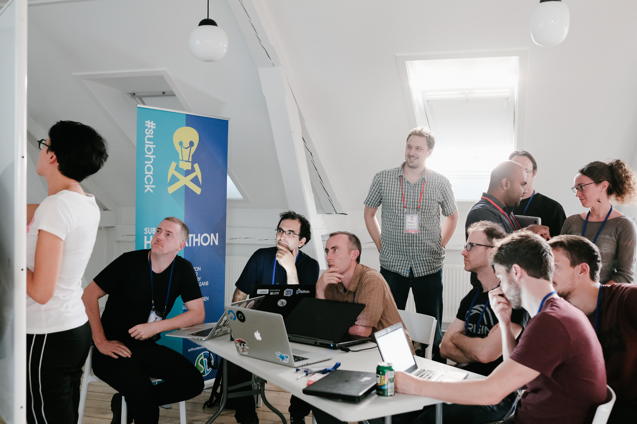
A code sprint is a type of hackathon, in which efforts are focused around a small number of open source projects. They are related to, but not really the same as, sprints in the Scrum software development framework. They are non-competitive — the only goal is to improve the software in question, whether it's adding functionality, fixing bugs, writing tests, improving documentation, or doing any of the other countless things that good software needs. 

On 13 and 14 October, we'll be hacking on 3 projects:

  • Devito: a high-level finite difference library for Python. Devito featured in three Geophysical Tutorials at the end of 2017 and beginning of 2018 (see Witte et al. for Part 3). The project needs help with code, tests, model examples, and documentation. There will be core devs from the project at the sprint. GitHub repo is here.
  • Bruges: a simple collection of Python functions representing basic geophysical equations. We built this library back in 2015, and have been chipping away ever since. It needs more equations, better docs, and better tests — and the project is basic enough for anyone to contribute to it, even a total Python newbie. GitHub repo is here.
  • G3.js: a JavaScript wrapper for D3.js, a popular plotting toolkit for web developers. When we tried to adapt D3.js to geoscience data, we found we wanted to simplify basic tasks like making vertical plots, and plotting raster-like data (e.g. seismic) with line plots on top (e.g. horizons). Experience with JavaScript is a must. GitHub repo is here.

The sprint will be at a small joint called MAZ Café Con Leche, located in Santa Ana about 10 km or 15 minutes from the Anaheim Convention Center where the SEG Annual Meeting is happening the following week.

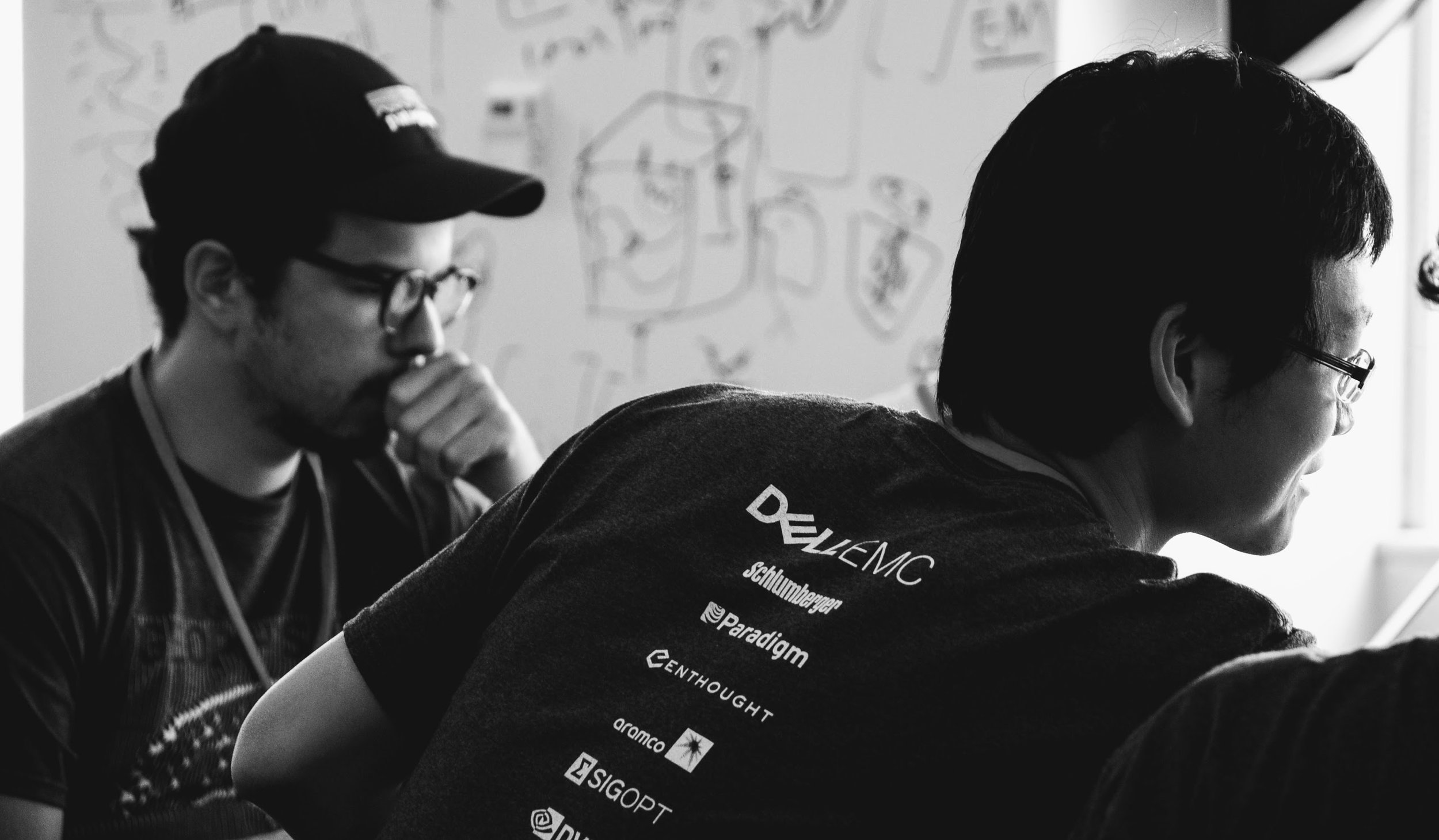
Thank you, as ever, to our fantastic sponsors: Dell EMC and Enthought. These two companies are powered by amazing people doing amazing things. I'm very grateful to them both for being such enthusiastic champions of the change we're working for in our science and our industry. 

If you like the sound of spending the weekend coding, talking geophysics, and enjoying the best coffee in southern California, please join us at the Geophysics Sprint! Register on Eventbrite and we'll see you there.

Visualization in Copenhagen, part 2

In Part 1, I wrote about six of the projects teams contributed at the Subsurface Hackathon in Copenhagen in June. Today I want to tell you about the rest of them. 


A data exploration tool

Team GeoClusterFu...n: Dan Stanton (University of Leeds), Filippo Broggini (ETH Zürich), Francois Bonneau (Nancy), Danny Javier Tapiero Luna (Equinor), Sabyasachi Dash (Cairn India), Nnanna Ijioma (geophysicist). 

Tech: Plotly Dash. GitHub repo.

Project: The team set out to build an interactive web app — a totally new thing for all of them — to make interactive plots from data in a CSV. They ended up with the basis of a useful tool for exploring geoscience data. Project page.

Four sixths of the GeoClusterFu...n team cluster around a laptop.

Four sixths of the GeoClusterFu...n team cluster around a laptop.


AR outcrop on your phone

Team SmARt_OGs: Brian Burnham (University of Aberdeen), Tala Maria Aabø (Natural History Museum of Denmark), Björn Wieczoreck, Georg Semmler and Johannes Camin (GiGa Infosystems).

Tech: ARKit/ARCore, WebAR, Firebase. GitLab repo. 

Project: Bjørn and his colleagues from GiGa Infosystems have been at all the European hackathons. This time, he knew he wanted to get virtual outcrops on mobiles phones. He found a willing team, and they got it done! Project page.

Three views from the SmartOGs's video. See the full version.

Three views from the SmartOGs's video. See the full version.


Rock clusters in latent space

The Embedders: Lukas Mosser (Imperial College London), Jesper Dramsch (Technical University of Denmark), Ben Fischer (PricewaterhouseCoopers), Harry McHugh (DUG), Shubhodip Konar (Cairn India), Song Hou (CGG), Peter Bormann (ConocoPhillips).

Tech: Bokeh, scikit-learn, Multicore-TSNE. GitHub repo.

Project: There has been a lot of recent interest in the t-SNE algorithm as a way to reduce the dimensionality of complex data. The team explored its application to subsurface data, and found promising applications. Web page. Project page.

The Embeders built a web app to cluster the data in an LAS file. The clusters (top left) are generated by the t-SNE algorithm.

The Embeders built a web app to cluster the data in an LAS file. The clusters (top left) are generated by the t-SNE algorithm.


Fully mixed reality

Team Hands On GeoLabs: Will Sanger (Western Geco), Chance Sanger (Houston Museum of Fine Arts), Pierre Goutorbe (Total), Fernando Villanueva (Institut de Physique du Globe de Paris).

Project: Starting with the ambitious goal of combining the mixed reality of the Meta AR gear with the mixed reality of the Gempy sandbox, the team managed to display and interact with some seismic data in the AR headset, which  allows interaction with simple hand gestures. Project page.

The team demonstrate the Meta AR headset.

The team demonstrate the Meta AR headset.


Huge grids over the web

Team Grid Vizards: Fabian Kampe, Daniel Buse, Jonas Kopcsek, Paul Gabriel (all from GiGa Infosystems)

Tech: three.js. GitHub repo.

Project: Paul and his team wanted to visualize hundreds of millions or billions of grid cells — all in the browser. They ended up with about 20 million points working very smoothly, and impressed everyone. Project page.

grid_vizards.png

Interpreting RGB displays for spec decomp

Team: Florian Smit (Technical University of Denmark), Gijs Straathof (SGS), Thomas Gazzola (Total), Julien Capgras (Total), Steve Purves (Euclidity), Tom Sandison (Shell)

Tech: Python, react.js. GitHub repos: Client. Backend.

Project: Spectral decomposition is still a mostly quantitative tool, especially the interpretation of RGB-blended displays. This team set out to make intuitive, attractive forward models of the spectral response of wells. This should help interpret seismic data, and perhaps make more useful RGB displays too. Intriguing and promising work. Project page.

RGB_log.png

That's it for another year! Twelve new geoscience visualization projects — ten of them open source. And another fun, creative weekend for 63 geoscientists — all of whom left with new connections and new skills. All this compressed into one weekend. If you haven't experienced a hackathon yet, I urge you to seek one out.

I will leave you with two videos — and an apology. We are so focused on creating a memorable experience for everyone in the room, that we tend to neglect the importance of capturing what's happening. Early hackathons only had the resulting blog post as the document of record, but lately we've been trying to livestream the demos at the end. Our success has been, er, mixed... but they were especially wonky this time because we didn't have livestream maestro Gram Ganssle there. So, these videos exist, and are part of the documentation of the event, but they barely begin to convey the awesomeness of the individuals, the teams, or their projects. Enjoy them, but next time — you should be there!

Visualization in Copenhagen, part 1

CPH_blog_banner.png

It's finally here! The round-up of projects from the Subsurface Hacakthon in Copenhagen last month. This is the first of two posts presenting the teams and their efforts, in the same random order the teams presented them at the end of the event.


Subsurface data meets Pokemon Go

Team Geo Go: Karine Schmidt, Max Gribner, Hans Sturm (all from Wintershall), Stine Lærke Andersen (University of Copenhagen), Ole Johan Hornenes (University of Bergen), Per Fjellheim (Emerson), Arne Kjetil Andersen (Emerson), Keith Armstrong (Dell EMC). 

Project: With Pokemon Go as inspiration, the team set out to prototype a geoscience visualization app that placed interactive subsurface data elements into a realistic 3D environment.

180610_agile_scientific_78.jpg

Visualizing blind spots in data

Team Blind Spots: Jo Bagguley (UK Oil & Gas Authority), Duncan Irving (Teradata), Laura Froelich (Teradata), Christian Hirsch (Aalborg University), Sean Walker (Campbell & Walker Geophysics).

Tech: Flask, Bokeh, AWS for hosting app. GitHub repo.

Project: Data management always comes up as an issue in conversations about geocomputing, but few are bold enough to tackle it head on. This team built components for checking the integrity of large amounts of raw data, before passing it to data science projects. Project page.

Sean, Laura, and Christian. Jo and Duncan were out doing research. Note the kanban board in the background — agile all the way!

Sean, Laura, and Christian. Jo and Duncan were out doing research. Note the kanban board in the background — agile all the way!


Volume uncertainties visualization

Team Fortuna: Natalia Shchukina (Total), Behrooz Bashokooh (Shell), Tobias Staal (University of Tasmania), Robert Leckenby (now Agile!), Graham Brew (Dynamic Graphics), Marco van Veen (RWTH Aachen). 

Tech: Flask, Bokeh, Altair, Holoviews. GitHub repo.

Project: Natalia brought some data with her: lots of surface grids. The team built a web app to compute uncertainty sections and maps, then display them dynamically and interactively — eliciting audible gasps from the room. Project page.

The Fortuna app: Probability of being the the zone (left) and entropy (right). Cross-sections are shown at the top, maps on the bottom.


Differences and similarities with RGB blends

Team RGBlend: Melanie Plainchault and Jonathan Gallon (Total), Per Olav Svendsen, Jørgen Kvalsvik and Max Schuberth (Equinor).

Tech: Python, Bokeh. GitHub repo.

Project: One of the more intriguing ideas of the hackathon was not just so much a fancy visualization technique, as a novel way of producing a visualization — differencing 3 images and visualizing the differences in RGB space. It reminded me of an old blog post about the spot the difference game. Project page.

The differences (lower right) between three time-lapse seismic amplitude maps.

The differences (lower right) between three time-lapse seismic amplitude maps.


Augmented reality geological maps

Team AR Sandbox: Simon Virgo (RWTH Aachen), Miguel de la Varga (RWTH Aachen), Fabian Antonio Stamm (RWTH Aachen), Alexander Schaaf (University of Aberdeen).

Tech: Gempy. GitHub repo.

Project: I don't have favourite projects, but if I did, this would be it. The GemPy group had already built their sandbox when they arrived, but they extended it during the hackathon. Wonderful stuff. Project page.

magic box of sand: Sculpting a landscape (left), and the projected map (right). You can't even imagine how much fun it was to play with.


Augmented reality seismic wavefields

Team Sandbox Seismics: Yuriy Ivanov (NTNU Trondheim), Ana Lim (NTNU Trondheim), Anton Kühl (University of Copenhagen), Jean Philippe Montel (Total).

Tech: GemPy, Devito. GitHub repo.

Project: This team worked closely with Team AR Sandbox, but took it in a different direction. They instead read the velocity from the surface of the sand, then used devito to simulate a seismic wavefield propagating across the model, and projected that wavefield onto the sand. See it in action in my recent Code Show post. Project page.

Yuriy Ivanov demoing the seismic wavefield moving across the sandbox.


Pretty cool, right? As usual, all of these projects were built during the hackathon weekend, almost exclusively by teams that formed spontaneously at the event itself (I think one team was self-contained from the start). If you didn't notice the affiliations of the participants — go back and check them out; I think this might have been an unprecedented level of collaboration!

Next time we'll look at the other six projects. [UPDATE: Next post is here.]

Before you go, check out this awesome video Wintershall made about the event. A massive thank you to them for supporting the event and for recording this beautiful footage — and for agreeing to share it under a CC-BY license. Amazing stuff!

Visualize this!

The Copenhagen edition of the Subsurface Hackathon is over! For three days during the warmest June in Denmark for over 100 years, 63 geoscientists and programmers cooked up hot code in the Rainmaking Loft, one of the coolest, and warmest, coworking spaces you've ever seen. As always, every one of the participants brought their A game, and the weekend flew by in a blur of creativity, coffee, and collaboration. And croissants.

Pierre enjoying the Meta AR headset that DEll EMC provided.

Pierre enjoying the Meta AR headset that DEll EMC provided.

Our sponsors have always been unusually helpful and inspiring, pushing us to get more audacious, but this year they were exceptionally engaged and proactive. Dell EMC, in the form of David and Keith, provided some fantastic tech for the teams to explore; Total supported Agile throughout the organization phase, and Wintershall kindly arranged for the event to be captured on film — something I hope to be able to share soon. See below for the full credit roll!

sponsors.png

During th event, twelve teams dug into the theme of visualization and interaction. As in Houston last September, we started the event on Friday evening, after the Bootcamp (a full day of informal training). We have a bit of process to form the teams, and it usually takes a couple of hours. But with plenty of pizza and beer for fuel, the evening flew by. After that, it was two whole days of coding, followed by demos from all of the teams and a few prizes. Check out some of the pictures:

Thank you very much to everyone that helped make this event happen! Truly a cast of thousands:

  • David Holmes of Dell EMC for unparallelled awesomeness.
  • The whole Total team, but especially Frederic Broust, Sophie Segura, Yannick Pion, and Laurent Baduel...
  • ...and also Arnaud Rodde for helping with the judging.
  • The Wintershall team, especially Andreas Beha, who also acted as a judge.
  • Brendon Hall of Enthought for sponsoring the event.
  • Carlos Castro and Kim Saabye Pedersen of Amazon AWS.
  • Mathias Hummel and Mahendra Roopa of NVIDIA.
  • Eirik Larsen of Earth Science Analytics for sponsoring the event and helping with the judging.
  • Duncan Irving of Teradata for sponsoring, and sorting out the T-shirts.
  • Monica Beech of Ikon Science for participating in the judging.
  • Matthias Hartung of Target for acting as a judge again.
  • Oliver Ranneries, plus Nina and Eva of Rainmaking Loft.
  • Christopher Backholm for taking such great photographs.

Finally, some statistics from the event:

  • 63 participants, including 8 women (still way too few, but 100% better than 4 out of 63 in Paris)
  • 15 students plus a handful of post-docs.
  • 19 people from petroleum companies.
  • 20 people from service and technology companies, including 7 from GiGa-infosystems!
  • 1 no-show, which I think is a new record.

I will write a summary of all the projects in a couple of weeks when I've caught my breath. In the meantime, you can read a bit about them on our new events portal. We'll be steadily improving this new tool over the coming weeks and months.

That's it for another year... except we'll be back in Europe before the end of the year. There's the FORCE Hackathon in Stavanger in September, then in November we'll be in Aberdeen and London running some events with the Oil and Gas Authority. If you want some machine learning fun, or are looking for a new challenge, please come along!

Simon Virgo (centre) and his colleagues in Aachen built an augmented reality sandbox, powered by their research group's software, Gempy. He brought it along and three teams attempted projects based on the technology. Above, some of the participants …

Simon Virgo (centre) and his colleagues in Aachen built an augmented reality sandbox, powered by their research group's software, Gempy. He brought it along and three teams attempted projects based on the technology. Above, some of the participants are having a scrum meeting to keep their project on track.


The right writing tools

Scientists write, it's part of the job. If writing feels laborious, it might be because you haven't found the right tools yet. 

The wrong tools <cough>Word</cough> feel like a lot of work. You spend a lot of time fiddling with font sizes and not being sure whether to use italic or bold. You're constantly renumbering sections after edits. Everything moves around when you resize a figure. Tables are a headache. Table of contents? LOL.

If this sounds familiar, check out the following tools — arranged more or less in order of complexity.

Markdown

If you've never experienced writing with a markup language, you're in for a treat. At first it might feel clunky, but it quickly gets out of the way, leaving you to focus on the writing. Markdown was invented by John Gruber in about 2004; it is now almost ubiquitous in tools for developers. It's very lightweight, but compatible with HTML and LaTeX math, so it has plenty of features. Styling is absent from the document itself, being applied enitrely in post-production, as it were. With help from pandoc, you can compile Markdown documents to almost any format (e.g. PDF or Word). As a result, Markdown is sufficient for at least 70% of my writing projects. Here's a sampling of Markdown markup, rendered on the right with no styling:

Markdown_raw.png
Markdown_render.png

Jupyter Notebook

If you've been following along with our X Lines of Python series, or any of our other code-centric content, you'll have come across Jupyter Notebooks. These documents combine Markdown with code (in more or less any language you can think of) and the outputs of code — data, charts, images, etc. More than containing code, a so-called kernel can also run the code: Notebooks are fully computable documents. Not only could you write a paper or book in a Notebook, many people use them to give presentations with fully interactive, live code blocks and widgets.

Notebook_example.png
latex_folder___by_missyobo-d3azzbh.png

LaTeX

I discovered LaTeX in about 1993 and it was love at first sight. I've always been a bit of a typography nerd, and LaTeX — like TeX, around which LaTeX is wrapped — really cares about typography. So you get ligatures, hyphenation, sentence spacing, and kerning for free. It also cares about mathematics, cross-references, bibliographies, page numbering, tables of contents, and everything else you need for publication-ready documents.

You can install LaTeX locally, but there are several ways to use LaTeX online, without installing anything — and you get the best of both worlds: markup with WYSIWYG editing. OverleafShareLaTex (which is merging with Overleaf), Authorea, and Papeeria are all worth a look, especially if you write scientific papers.

When WYSISYG works

Sometimes you just want a couple of headings and some text, or you need to share a document with others. I often go for WYSISYG in those situations too — Google Docs is the best WYSIWYG editor I've used. When it supports Markdown too, which is surely only a matter of time, it will be perfect.

What about you, do you have a favourite writing tool? Share it in the comments.

Easier, better, faster, stronger

bruges_preview_1.png

Yesterday I pushed a new release of bruges to Python's main package repository, PyPi.  Version 0.3.3 might not sound like an especially auspicious version perhaps, but I'm excited about the new things we've added recently. It has come a long way since we announced it back in 2015, so if you haven't checked it out lately, now's a good time to take another look.

What is bruges again?

Bruges is a...

In other words, nothing fancy — just equations. It is free, open source software. It's aimed at geophysicists who use Python.

How do you install it? The short answer is pip:

    pip install bruges

So what's new?

Here are the highlights of what's been improved and added in the last few months:

  • The reflectivity equations in reflection module now work on arrays for the Vp, Vs, and rho values, as well as the theta values. This is about 10 times faster than running a loop over elements; the Zoeppritz solution is 100× faster.
  • The various Zoeppritz solutions and the Aki–Richards approximations now return the complex reflectivity and therefore show post-critical amplitudes correctly.
  • A new reflection coefficient series function, reflection.reflectivity(), makes it easier to compute offset reflectivities from logs.
  • Several new linear and non-linear filters are in bruges.filters, including median (good for seismic horizons), mode (good for waveform classification), symmetric nearest-neighbours or snn, and kuwahara.
  • The wavelets ricker(), sweep() (aka Klauder) and ormsby() wavelet now all work for a sequence of frequencies, returning a wavelet bank. Also added a sinc() wavelet, with a taper option to attenuate the sidelobes.
  • Added inverse_gardner, and other density and velocity transforms, to petrophysics.
  • Added transform.v_rms() (RMS velocity), transform.v_avg() (average velocity) and transform.v_bac() (naïve Backus average). These all operate in a 'cumulative' average-down-to sense.
  • Added a coordinate transformation to translate between arbitrarily oriented (x,y) and (inline, line) coordinates.

Want to try using it right now, with no installation? Give it a spin in My Binder! See how easy it is to compute elastic moduli, or offset reflection coefficients, or convert a log to time.  

bruges_preview_2.png

Want to support the development of open source geophysics software? Here's how:

  • Use it! This is the main thing we care about.
  • Report problems on the project's Issue page.
  • Fork the project and make your own changes, then share them back.
  • Pay us for the development of functionality you need.

x lines of Python: Let's play golf!

Normally in the x lines of Python series, I'm trying to do something useful in as few lines of code as possible, but — and this is important — without sacrificing clarity. Code golf, on the other hand, tries solely to minimize the number of characters used, and to heck with clarity. This might, and probably will, result in rather obfuscated code.

So today in x lines, we set x = 1 and see what kind of geophysics we can express. Follow along in the accompanying notebook if you like.

A Ricker wavelet

One of the basic building blocks of signal processing and therefore geophysics, the Ricker wavelet is a compact, pulse-like signal, often employed as a source in simulation of seismic and ground-penetrating radar problems. Here's the equation for the Ricker wavelet:

$$ A = (1-2 \pi^2 f^2 t^2) e^{-\pi^2 f^2 t^2} $$

where \(A\) is the amplitude at time \(t\), and \(f\) is the centre frequency of the wavelet. Here's one way to translate this into Python, more or less as expressed on SubSurfWiki:

import numpy as np 
def ricker(length, dt, f):
    """Ricker wavelet at frequency f Hz, length and dt in seconds.
    """
    t = np.arange(-length/2, length/2, dt)
    y = (1.0 - 2.0*(np.pi**2)*(f**2)*(t**2)) * np.exp(-(np.pi**2)*(f**2)*(t**2))
    return t, y

That is alredy pretty terse at 261 characters, but there are lots of obvious ways, and some non-obvious ways, to reduce it. We can get rid of the docstring (the long comment explaining what the function does) for a start. And use the shortest possible variable names. Then we can exploit the redundancy in the repeated appearance of \(\pi^2f^2t^2\)... eventually, we get to:

def r(l,d,f):import numpy as n;t=n.arange(-l/2,l/2,d);k=(n.pi*f*t)**2;return t,(1-2*k)/n.exp(k)

This weighs in at just 95 characters. Not a bad reduction from 261, and it's even not too hard to read. In the notebook accompanying this post, I check its output against the version in our geophysics package bruges, and it's legit:

The 95-character Ricker wavelet in green, with the points computed by the function in BRuges.

The 95-character Ricker wavelet in green, with the points computed by the function in BRuges.

What else can we do?

In the notebook for this post, I run through some more algorithms for which I have unit-tested examples in bruges:

To give you some idea of why we don't normally code like this, here's what the Aki–Richards solution looks like:

def r(a,c,e,b,d,f,t):import numpy as n;w=f-e;x=f+e;y=d+c;p=n.pi*t/180;s=n.sin(p);return w/x-(y/a)**2*w/x*s**2+(b-a)/(b+a)/n.cos((p+n.arcsin(b/a*s))/2)**2-(y/a)**2*(2*(d-c)/y)*s**2

A bit hard to debug! But there is still some point to all this — I've found I've had to really understand Python's order of mathematical operations, and find different ways of doing familiar things. Playing code golf also makes you think differently about repetition and redundancy. All good food for developing the programming brain.

Do have a play with the notebook, which you can even run in Microsoft Azure, right in your browser! Give it a try. (You'll need an account to do this. Create one for free.)


Many thanks to Jesper Dramsch and Ari Hartikainen for helping get my head into the right frame of mind for this silliness!

A new blog, and a new course

There's a great new geoscience blog on the Internet — I urge you to add it to your blog-reading app or news reader or list of links or whatever it is you use to keep track of these things. It's called Geology and Python, and it contains exactly what you'd expect it to contain!

The author, Bruno Ruas de Pinho, has nine posts up so far, all excellent. The range of topics is quite broad:

In each post, Bruno takes some geoscience challenge — nothing too huge, but the problems aren't trivial either — and then methodically steps through solving the problem in Python. He's clearly got a good quantitative brain, having recently graduated in geological engineering from the Federal University of Pelotas, aka UFPel, Brazil, and he is now available for hire. (He seems to be pretty sharp, so if you're doing anything with computers and geoscience, you should snag him.)


A new course for Calgary

We've run lots of Introduction to Python courses before, usually with the name Creative Geocomputing. Now we're adding a new dimension, combining a crash introduction to Python with a crash introduction to machine learning. It's ambitious, for sure, but the idea is not to turn you into a programmer. We aim to:

  • Help you set up your computer to run Python, virtual environments, and Jupyter Notebooks.
  • Get you started with downloading and running other people's packages and notebooks.
  • Verse you in the basics of Python and machine learning so you can start to explore.
  • Set you off with ideas and things to figure out for that pet project you've always wanted to code up.
  • Introduce you to other Calgarians who love playing with code and rocks.

We do all this wielding geoscientific data — it's all well logs and maps and seismic data. There are no silly examples, and we don't shy away from so-called advanced things — what's the point in computers if you can't do some things that are really, really hard to do in your head?

Tickets are on sale now at Eventbrite, it's $750 for 2 days — including all the lunch and code you can eat.

Hacking in Houston

geohack_2017_banner.png

Houston 2013
Houston 2014
Denver 2014
Calgary 2015
New Orleans 2015
Vienna 2016
Paris 2017
Houston 2017... The eighth geoscience hackathon landed last weekend!

We spent last weekend in hot, humid Houston, hacking away with a crowd of geoscience and technology enthusiasts. Thirty-eight hackers joined us on the top-floor coworking space, Station Houston, for fun and games and code. And tacos.

Here's a rundown of the teams and what they worked on.

Seismic Imagers

Jingbo Liu (CGG), Zohreh Souri (University of Houston).

Tech — DCGAN in Tensorflow, Amazon AWS EC2 compute.

The team looked for patterns that make seismic data different from other images, using a deep convolutional generative adversarial network (DCGAN). Using a seismic volume and a set of 2D lines, they made 121,000 sub-images (tiles) for their training set.

The Young And The RasLAS

William Sanger (Schlumberger), Chance Sanger (Museum of Fine Arts, Houston), Diego Castañeda (Agile), Suman Gautam (Schlumberger), Lanre Aboaba (University of Arkansas).

State of the art text detection by Google Cloud Vision API

State of the art text detection by Google Cloud Vision API

Tech — Google Cloud Vision API, Python flask web app, Scatteract (sort of). Repo on GitHub.

Digitizing well logs is a common industry task, and current methods require a lot of manual intervention. The team's automated pipeline: convert PDF files to images, perform OCR with Google Cloud Vision API to extract headers and log track labels, pick curves using a CNN in TensorFlow. The team implemented the workflow in a Python flask front-end. Check out their slides.

Hutton Rocks

Kamal Hami-Eddine (Paradigm), Didi Ooi (University of Bristol), James Lowell (GeoTeric), Vikram Sen (Anadarko), Dawn Jobe (Aramco).

hutton.png

Tech — Amazon Echo Dot, Amazon AWS (RDS, Lambda).

The team built Hutton, a cloud-based cognitive assistant for gaining more efficient, better insights from geologic data. Project includes integrated cloud-hosted database, interactive web application for uploading new data, and a cognitive assistant for voice queries. Hutton builds upon existing Amazon Alexa skills. Check out their GitHub repo, and slides.

Big data > Big Lore 

Licheng Zhang (CGG), Zhenzhen Zhong (CGG), Justin Gosses (Valador/NASA), Jonathan Parker (Marathon)

The team used machine learning to predict formation tops on wireline logs, which would allow for rapid generation of structure maps for exploration play evaluation, save man hours and assist in difficuly formation-top correlations. The team used the AER Athabasca open dataset of 2193 wells (yay, open data!).

Tech — Jupyter Notebooks, SciPy, scikit-learn. Repo on GitHub.

Free near surface

free_surface.png

Tien-Huei Wang, Jing Wu, Clement Zhang (Schlumberger).

Multiples are a kind of undesired seismic signal and take expensive modeling to remove. The project used machine learning to identify multiples in seismic images. They attempted to use GAN frameworks, but found it difficult to formulate their problem, turning instead to the simpler problem of binary classification. Check out their slides.

Tech — CNN... I don't know the framework.

The Cowboyz

Mingliang Liu, Mohit Ayani, Xiaozheng Lang, Wei Wang (University of Wyoming), Vidal Gonzalez (Universidad Simón Bolívar, Venezuela).

A tight group of researchers joined us from the University of Wyoming at Laramie, and snagged one of the most enthusiastic hackers at the event, a student from Venezuela called Vidal. The team attempted acceleration of geostatistical seismic inversion using TensorFlow, a central theme in Mingliang's research.

Tech — TensorFlow.

Augur.ai

Altay Sensal (Geokinetics), Yan Zaretskiy (Aramco), Ben Lasscock (Geokinetics), Colin Sturm (Apache), Brendon Hall (Enthought).

augur.ai.JPG

Electrical submersible pumps (ESPs) are critical components for oil production. When they fail, they can cause significant down time. Augur.ai provides tools to analyze pump sensor data to predict when pumps when pump are behaving irregularly. Check out their presentation!

Tech — Amazon AWS EC2 and EFS, Plotly Dash, SigOpt, scikit-learn. Repo on GitHub.

disaster_input.png

The Disaster Masters

Joe Kington (Planet), Brendan Sullivan (Chevron), Matthew Bauer (CSM), Michael Harty (Oxy), Johnathan Fry (Chevron)

Hydrologic models predict floodplain flooding, but not local street flooding. Can we predict street flooding from LiDAR elevation data, conditioned with citizen-reported street and house flooding from U-Flood? Maybe! Check out their slides.

Tech — Python geospatial and machine learning stacks: rasterio, shapely, scipy.ndimage, scikit-learn. Repo on GitHub.

The structure does WHAT?!

Chris Ennen (White Oak), Nanne Hemstra (dGB Earth Sciences), Nate Suurmeyer (Shell), Jacob Foshee (Durwella).

Inspired by the concept of an iPhone 'face ageing' app, Nate recruited a team to poke at applying the concept to maps of the subsurface. Think of a simple map of a structural field early in its life, compared to how it looks after years of interpretation and drilling. Maybe we can preview the 'aged' appearance to help plan where best to drill next to reduce uncertainty!

Tech — OpendTect, Azure ML Studio, C#, self-boosting forest cluster. Repo on GitHub.


Thank you!

Massive thanks to our sponsors — including Pioneer Natural Resources — for their part in bringing the event to life! 

sponsors_tight.png

More thank-yous

Apart from the participants themselves, Evan and I benefitted from a team of technical support, mentors, and judges — huge thanks to all these folks:

  • The indefatigable David Holmes from Dell EMC. The man is a legend.
  • Andrea Cortis from Pioneer Natural Resources.
  • Francois Courteille and Issam Said of NVIDIA.
  • Carlos Castro, Sunny Sunkara, Dennis Cherian, Mike Lapidakis, Jit Biswas, and Rohan Mathews of Amazon AWS.
  • Maneesh Bhide and Steven Tartakovsky of SigOpt.
  • Dave Nichols and Aria Abubakar of Schlumberger.
  • Eric Jones from Enthought.
  • Emmanuel Gringarten from Paradigm.
  • Frances Buhay and Brendon Hall for help with catering and logistics.
  • The team at Station for accommodating us.
  • Frank's Pizza, Tacos-a-Go-Go, Cali Sandwich (banh mi), Abby's Cafe (bagels), and Freebird (burritos) for feeding us.

Finally, megathanks to Gram Ganssle, my Undersampled Radio co-host. Stalwart hack supporter and uber-fixer, Gram came over all the way from New Orleans to help teams make sense of deep learning architectures and generally smooth things over. We recorded an episode of UR at the hackathon, talking to Dawn Jobe, Joe Kington, and Colin Sturm about their respective projects. Check it out!


[Update, 29 Sep & 3 Nov] Some statistics from the event:

  • 39 participants, including 7 women (way too few, but better than 4 out of 63 in Paris)
  • 9 students (and 0 professors!).
  • 12 people from petroleum companies.
  • 18 people from service and technology companies, including 5 from Schlumberger!
  • 13 no-shows, not including folk who cancelled ahead of time; a bit frustrating because we had a long wait list.
  • Furthest travelled: James Lowell from Newcastle, UK — 7560 km!
  • 98 tacos, 67 burritos, 96 slices of pizza, 55 kolaches, and an untold number of banh mi.

Organizing spreadsheets

A couple of weeks ago I alluded to ill-formed spreadsheets in my post Murphy's Law for Excel. Spreadsheets are clearly indispensable, and are definitely great for storing data and checking CSV files. But some spreadsheets need to die a horrible death. I'm talking about spreadsheets that look like this (click here for the entire sheet):

Bad_spreadsheet_3.png

This spreadsheet has several problems. Among them:

  • The position of a piece of data changes how I interpret it. E.g. a blank row means 'new sheet' or 'new well'.
  • The cells contain a mixture of information (e.g. 'Site' and the actual data) and appear in varying units.
  • Some information is encoded by styles (e.g. using red to denote a mineral species). If you store your sheet as a CSV (which you should), this information will be lost.
  • Columns are hidden, there are footnotes, it's just a bit gross.

Using this spreadsheet to make plots, or reading it with software, with be a horrible experience. I will probably swear at my computer, suffer a repetitive strain injury, and go home early with a headache, cursing the muppet that made the spreadsheet in the first place. (Admittedly, I am the muppet that made this spreadsheet in this case, but I promise I did not invent these pathologies. I have seen them all.)

Let's make the world a better place

Consider making separate sheets for the following:

  • Raw data. This is important. See below.
  • Computed columns. There may be good reasons to keep these with the data.
  • Charts.
  • 'Tabulated' data, like my bad spreadsheet above, with tables meant for summarization or printing.
  • Some metadata, either in the file properties or a separate sheet. Explain the purpose of the dataset, any major sources, important assumptions, and your contact details.
  • A rich description of each column, with its caveats and assumptions.

The all-important data sheet has its own special requirements. Here's my guide for a pain-free experience:

  • No computed fields or plots in the data sheet.
  • No hidden columns.
  • No semantic meaning in formatting (e.g. highlighting cells or bolding values).
  • Headers in the first row, only data in all the other rows.
  • The column headers should contain only a unique name and [units], e.g. Depth [m], Porosity [v/v].
  • Only one type of data per column: text OR numbers, discrete categories OR continuous scalars.
  • No units in numeric data cells, only quantities. Record depth as 500, not 500 m.
  • Avoid keys or abbreviations: use Sandstone, Limestone, Shale, not Ss, Ls, Sh.
  • Zero means zero, empty cell means no data.
  • Only one unit per column. (You only use SI units right?)
  • Attribution! Include a citation or citations for every record.
  • If you have two distinct types or sources of data, e.g. grain size from sieve analysis and grain size from photomicrographs, then use two different columns.
  • Personally, I like the data sheet to be the first sheet in the file, but maybe that's just me.
  • Check that it turns into a valid CSV so you can use this awesome format.

      After all that, here's what we have (click here for the entire sheet):

    The same data as the first image, but improved. The long strings in columns 3 and 4 are troublesome, but we can tolerate them. Click to enlarge.

    Maybe the 'clean' analysis-friendly sheet looks boring to you, but to me it looks awesome. Above all, it's easy to use for SCIENCE! And I won't have to go home with a headache.


    The data in this post came from this Cretaceous shale dataset [XLS file] from the government of Manitoba. Their spreadsheet is pretty good and only breaks a couple of my golden rules. Here's my version with the broken and fixed spreadsheets shown here. Let me know if you spot something else that should be fixed!