Relentlessly practical

This is one of my favourite knowledge sharing stories.

A farmer in my community had a problem with one of his cows — it was seriously unwell. He asked one of the old local farmers about the symptoms, and was told, “Oh yes, one of my herd had the same thing last summer. I gave her a cup of brandy and four aspirins every night for a week.” The young farmer went off and did this, but the poor cow got steadily worse and died. When he saw the old farmer next he told him, more than a little accusingly, “I did what you said, and the cow died anyway.” The old geezer looked into the distance and just said, “Yep, so did mine.”

Incomplete information can be less useful than no information. Yet incomplete information has somehow become our specialty in applied geoscience. How often do we share methods, results, or case studies without the critical details that would make it useful information? That is, not just marketing, or resumé padding. Inded, I heard this week that one large US operator will not approve a publication that does include these critical details! And we call ourselves scientists...

Completeness mandatory

Thankfully, Last month The Leading Edge — the magazine of the SEG — started a new tutorial column, edited by me. Well, I say 'edited', I'm just the person that pesters prospective authors until they give in and send me a manuscript. Tad Smith, Don Herron, and Jenny Kucera are the people that make it actually happen. But I get to take all the credit.

When I was asked about it, I suggested two things:

  1. Make each tutorial reproducible by publishing the code that makes the figures.
  2. Make the words, the data, and the code completely open and shareable. 

To my delight and, I admit, slight surprise, they said 'Sure!'. So the words are published under an open license (Creative Commons Attribution-ShareAlike, the same license for re-use that most of Wikipedia has), the tutorials use open data for everything, and the code is openly available and free to re-use. Complete transparency.

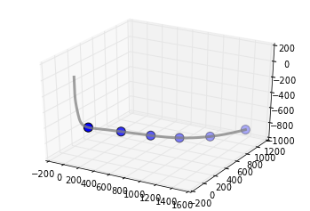
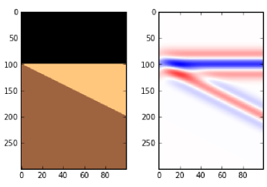
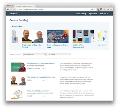
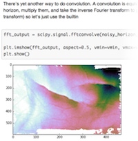
There's another interesting aspect to how the column is turning out. The first two episodes tell part of the story in IPython Notebook, a truly amazing executable writing environment that we've written about before. This enables you to seamlessly stich together text, code, and plots (left). If you know a bit of Python, or want to start learning it right now this second, go give wakari.io a try. It's pretty great. (If you really like it, come and learn more with us!).

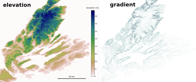
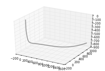
Read the first tutorial: Hall, M. (2014). Smoothing surfaces and attributes. The Leading Edge, 33(2), 128–129. doi: 10.1190/tle33020128.1. A version of it is also on SEG Wiki, and you can read the IPython Notebook at nbviewer.org.

Do you fancy authoring something for this column? Wonderful — please do! Here are the author instructions. If you have an idea for something, please drop me a line, let's talk about how to make it relentlessly practical.

Creating in the classroom

The day before the Atlantic Geoscience Colloquium, I hosted a one-day workshop on geoscience computing to 26 maritime geoscientists. This was my third time running this course. Each time it has needed tailoring and new exercises to suit the crowd; a room full of signal-processing seismologists has a different set of familiarities than one packed with hydrologists, petrologists, and cartographers. 

Easier to consume than create

At the start of the day, I asked people to write down the top five things they spend time doing with computers. I wanted a record of the tools people use, but also to take collective stock of our creative, as opposed to consumptive, work patterns. Here's the result (right).

My assertion was that even technical people spend most of their time in relatively passive acts of consumption — browsing, emailing, and so on. Creative acts like writing, drawing, or using software were in the minority, and only a small sliver of time is spent programming. Instead of filing into a darkened room and listening to PowerPoint slides, or copying lectures notes from a chalkboard, this course was going to be different. Participation mandatory.

My goal is not to turn every geoscientist into a software developer, but to better our capacity to communicate with computers. Giving people resources and training to master this medium that warrants a new kind of creative expression. Through coaching, tutorials, and exercises, we can support and encourage each other in more powerful ways of thinking. Moreover, we can accelerate learning, and demystify computer programming by deliberately designing exercises that are familiar and relevant to geoscientists. 

Scientific computing

In the first few hours students learned about syntax, built-in functions, how and why to define and call functions, as well as how to tap into external code libraries and documentation. Scientific computing is not necessarily about algorithm theory, passing unit tests, or designing better user experiences. Scientists are above all interested in data, and data processes, helped along by rich graphical displays for story telling.

Elevation model (left), and slope magnitude (right), Cape Breton, Nova Scotia. Click to enlarge.

In the final exercise of the afternoon, students produced a topography map of Nova Scotia (above left) from a georeferenced tiff. Sure, it's the kind of thing that can be done with a GIS, and that is precisely the point. We also computed some statistical properties to answer questions like, "what is the average elevation of the province?", or "what is the steepest part of the province?". Students learned about doing calculus on surfaces as well as plotting their results. 

Programming is a learnable skill through deliberate practice. What's more, if there is one thing you can teach yourself on the internet, it is computer programming. Perhaps what is scarce though, is finding the time to commit to a training regimen. It's rare that any busy student or working professional can set aside a chunk of 8 hours to engage in some deliberate coaching and practice. A huge bonus is to do it alongside a cohort of like-minded individuals willing and motivated to endure the same graft. This is why we're so excited to offer this experience — the time, help, and support to get on with it.

How can I take the course?

We've scheduled two more episodes for the spring, conveniently aligned with the 2014 AAPG convention in Houston, and the 2014 CSPG / CSEG convention in Calgary. It would be great to see you there!

Eventbrite - Agile Geocomputing  Eventbrite - Agile Geocomputing

Or maybe a customized in-house course would suit your needs better? We'd love to help. Get in touch.

To make up microseismic

I am not a proponent of making up fictitious data, but for the purposes of demonstrating technology, why not? This post is the third in a three-part follow-up from the private beta I did in Calgary a few weeks ago. You can check out the IPython Notebook version too. If you want more of this in person, sign up at the bottom or drop us a line. We want these examples to be easily readable, especially if you aren't a coder, so please let us know how we are doing.

Start by importing some packages that you'll need into the workspace,

%pylab inline
import numpy as np
from scipy.interpolate import splprep, splev
import matplotlib.pyplot as plt
import mayavi.mlab as mplt
from mpl_toolkits.mplot3d import Axes3D

Define a borehole path

We define the trajectory of a borehole, using a series of x, y, z points, and make each component of the borehole an array. If we had a real well, we load the numbers from the deviation survey just the same.

trajectory = np.array([[   0,   0,    0],
                       [   0,   0, -100],
                       [   0,   0, -200],
                       [   5,   0, -300],
                       [  10,  10, -400],
                       [  20,  20, -500],
                       [  40,  80, -650],
                       [ 160, 160, -700],
                       [ 600, 400, -800],
                       [1500, 960, -800]])
x = trajectory[:,0]
y = trajectory[:,1]
z = trajectory[:,2]

But since we want the borehole to be continuous and smoothly shaped, we can up-sample the borehole by finding the B-spline representation of the well path,

smoothness = 3.0
spline_order = 3
nest = -1 # estimate of number of knots needed (-1 = maximal)
knot_points, u = splprep([x,y,z], s=smoothness, k=spline_order, nest=-1)

# Evaluate spline, including interpolated points
x_int, y_int, z_int = splev(np.linspace(0, 1, 400), knot_points)

plt.gca(projection='3d')
plt.plot(x_int, y_int, z_int, color='grey', lw=3, alpha=0.75)
plt.show()

Define frac ports

Let's define a completion program so that our wellbore has 6 frac stages,

number_of_fracs = 6

and let's make it so that each one emanates from equally spaced frac ports spanning the bottom two-thirds of the well.

x_frac, y_frac, z_frac = splev(np.linspace(0.33, 1, number_of_fracs), knot_points)

Make a set of 3D axes, so we can plot the well path and the frac ports.

ax = plt.axes(projection='3d')
ax.plot(x_int, y_int, z_int, color='grey',
        lw=3, alpha=0.75)
ax.scatter(x_frac, y_frac, z_frac,
        s=100, c='grey')
plt.show()

Set a colour for each stage by cycling through red, green, and blue,

stage_color = []
for i in np.arange(number_of_fracs):
    color = (1.0, 0.1, 0.1)
    stage_color.append(np.roll(color, i))
stage_color = tuple(map(tuple, stage_color))

Define microseismic points

One approach is to create some dimensions for each frac stage and generate 100 points randomly within each zone. Each frac has an x half-length, y half-length, and z half-length. Let's also vary these randomly for each of the 6 stages. Define the dimensions for each stage:

frac_dims = []
half_extents = [500, 1000, 250]
for i in range(number_of_fracs):
    for j in range(len(half_extents)):
        dim = np.random.rand(3)[j] * half_extents[j]
        frac_dims.append(dim)  
frac_dims = np.reshape(frac_dims, (number_of_fracs, 3))

Plot microseismic point clouds with 100 points for each stage. The following code should launch a 3D viewer scene in its own window:

size_scalar = 100000
mplt.plot3d(x_int, y_int, z_int, tube_radius=10)
for i in range(number_of_fracs):
    x_cloud = frac_dims[i,0] * (np.random.rand(100) - 0.5)
    y_cloud = frac_dims[i,1] * (np.random.rand(100) - 0.5)
    z_cloud = frac_dims[i,2] * (np.random.rand(100) - 0.5)

    x_event = x_frac[i] + x_cloud
    y_event = y_frac[i] + y_cloud     
    z_event = z_frac[i] + z_cloud
    
    # Let's make the size of each point inversely proportional 
    # to the distance from the frac port
    size = size_scalar / ((x_cloud**2 + y_cloud**2 + z_cloud**2)**0.002)
    
    mplt.points3d(x_event, y_event, z_event, size, mode='sphere', colormap='jet')

You can swap out the last line in the code block above with mplt.points3d(x_event, y_event, z_event, size, mode='sphere', color=stage_color[i]) to colour each event by its corresponding stage.

A day of geocomputing

I will be in Calgary in the new year and running a one-day version of this new course. To start building your own tools, pick a date and sign up:

Eventbrite - Agile Geocomputing    Eventbrite - Agile Geocomputing

To make a wedge

We'll need a wavelet like the one we made last time. We could import it, if we've made one, but SciPy also has one so we can save ourselves the trouble. Remember to put %pylab inline at the top if using IPython notebook.

import numpy as np
from scipy.signal import ricker
import matplotlib.pyplot as plt

Now we need to make a physical earth model with three rock layers. In this example, let's make an acoustic impedance earth model. To keep it simple, let's define the earth model with two-way-travel time along the vertical axis (as opposed to depth). There are number of ways you could describe a wedge using math, and you could probably come up with a way that is better than mine. Here's a way:

nsamps, ntraces = [600, 500]
rock_names = ['shale 1', 'sand', 'shale 2']
rock_grid = np.zeros((n_samples, n_traces))

def make_wedge(n_samples, n_traces, layer_1_thickness, start_wedge, end_wedge):
    for j in np.arange(n_traces): 
        for i in np.arange(n_samples):      
            if i <= layer_1_thickness:      
rock_grid[i][j] = 1 if i > layer_1_thickness:
rock_grid[i][j] = 3 if j >= start_wedge and i - layer_1_thickness < j-start_wedge:
rock_grid[i][j] = 2 if j >= end_wedge and i > layer_1_thickness+(end_wedge-start_wedge):
rock_grid[i][j] = 3 return rock_grid

Let's insert some numbers into our wedge function and make a particular geometry.

layer_1_thickness = 200
start_wedge = 50
end_wedge = 250
rock_grid = make_wedge(n_samples, n_traces, 
            layer_1_thickness, start_wedge, 
            end_wedge)

plt.imshow(rock_grid, cmap='copper_r')

Now we can give each layer in the wedge properties.

vp = np.array([3300., 3200., 3300.]) 
rho = np.array([2600., 2550., 2650.]) 
AI = vp*rho
AI = AI / 10e6 # re-scale (optional step)

Then assign values assign them accordingly to every sample in the rock model.

model = np.copy(rock_grid)
model[rock_grid == 1] = AI[0]
model[rock_grid == 2] = AI[1]
model[rock_grid == 3] = AI[2]
plt.imshow(model, cmap='Spectral')
plt.colorbar()
plt.title('Impedances')

Now we can compute the reflection coefficients. I have left out a plot of the reflection coefficients, but you can check it out in the full version in the nbviewer

upper = model[:-1][:]
lower = model[1:][:]
rc = (lower - upper) / (lower + upper)
maxrc = abs(np.amax(rc))

Now we make the wavelet interact with the model using convolution. The convolution function already exists in the SciPy signal library, so we can just import it.

from scipy.signal import convolve
def make_synth(f):
    synth = np.zeros((n_samples+len(t)-2, n_traces))
    wavelet = ricker(512, 1e3/(4.*f))
    wavelet = wavelet / max(wavelet)   # normalize
    for k in range(n_traces):
        synth[:,k] = convolve(rc[:,k], wavelet)
    synth = synth[ np.ceil(len(wavelet))/2 : -np.ceil(len(wavelet))/2, : ]
    return synth

Finally, we plot the results.

frequencies = array([5, 10, 15]) plt.figure(figsize = (15, 4)) for i in np.arange(len(frequencies)): this_plot = make_synth(frequencies[i]) plt.subplot(1, len(frequencies), i+1) plt.imshow(this_plot, cmap='RdBu', vmax=maxrc, vmin=-maxrc, aspect=1) plt.title( '%d Hz wavelet' % freqs[i] ) plt.grid() plt.axis('tight') # Add some labels for i, names in enumerate(rock_names): plt.text(400, 100+((end_wedge-start_wedge)*i+1), names, fontsize=14, color='gray', horizontalalignment='center', verticalalignment='center')


That's it. As you can see, the marriage of building mathematical functions and plotting them can be a really powerful tool you can apply to almost any physical problem you happen to find yourself working on.

You can access the full version in the nbviewer. It has a few more figures than what is shown in this post.

A day of geocomputing

I will be in Calgary in the new year and running a one-day version of this new course. To start building your own tools, pick a date and sign up:

Eventbrite - Agile Geocomputing    Eventbrite - Agile Geocomputing

To plot a wavelet

As I mentioned last time, a good starting point for geophysical computing is to write a mathematical function describing a seismic pulse. The IPython Notebook is designed to be used seamlessly with Matplotlib, which is nice because we can throw our function on graph and see if we were right. When you start your own notebook, type

ipython notebook --pylab inline

We'll make use of a few functions within NumPy, a workhorse to do the computational heavy-lifting, and Matplotlib, a plotting library.

import numpy as np
import matplotlib.pyplot as plt

Next, we can write some code that defines a function called ricker. It computes a Ricker wavelet for a range of discrete time-values t and dominant frequencies, f:

def ricker(f, length=0.512, dt=0.001):
    t = np.linspace(-length/2, (length-dt)/2, length/dt)
    y = (1.-2.*(np.pi**2)*(f**2)*(t**2))*np.exp(-(np.pi**2)*(f**2)*(t**2))
    return t, y

Here the function needs 3 input parameters; frequency, f, the length of time over which we want it to be defined, and the sample rate of the signal, dt. Calling the function returns two arrays, the time axis t, and the value of the function, y.

To create a 5 Hz Ricker wavelet, assign the value of 5 to the variable f, and pass it into the function like so,

f = 5
t, y = ricker (f)

To plot the result,

plt.plot(t, y)

But with a few more commands, we can improve the cosmetics,

plt.figure(figsize=(7,4))
plt.plot( t, y, lw=2, color='black', alpha=0.5)
plt.fill_between(t, y, 0,  y > 0.0, interpolate=False, hold=True, color='blue', alpha = 0.5)
plt.fill_between(t, y, 0, y < 0.0, interpolate=False, hold=True, color='red', alpha = 0.5)

# Axes configuration and settings (optional)
plt.title('%d Hz Ricker wavelet' %f, fontsize = 16 )
plt.xlabel( 'two-way time (s)', fontsize = 14)
plt.ylabel('amplitude', fontsize = 14)
plt.ylim((-1.1,1.1))
plt.xlim((min(t),max(t)))
plt.grid()
plt.show()

Next up, we'll make this wavelet interact with a model of the earth using some math. Let me know if you get this up and running on your own.

Let's do it

It's short notice, but I'll be in Calgary again early in the new year, and I will be running a one-day version of this new course. To start building your own tools, pick a date and sign up:

Eventbrite - Agile Geocomputing    Eventbrite - Agile Geocomputing

Coding to tell stories

Last week, I was in Calgary on family business, but I took an afternoon to host a 'private beta' for a short course that I am creating for geoscience computing. I invited about twelve familiar faces who would be provide gentle and constuctive feedback. In the end, thirteen geophysicists turned up, seven of whom I hadn't met before. So much for familiarity.

I spent about two and half hours stepping through the basics of the Python programming language, which I consider essential material — getting set up with Python via Enthought Canopy, basic syntax, and so on. In the last hour of the afternoon, I steamed through a number of geoscientific examples to showcase exercises for this would-be course. 

Here are three that went over well. Next week, I'll reveal the code for making these images. I might even have a go at converting some of my teaching materials from IPython Notebook to HTML:

To plot a wavelet

The Ricker wavelet is a simple analytic function that is used throughout seismology. This curvaceous waveform is easily described by a single variable, the dominant frequency of its many contituents frequencies. Every geophysicist and their cat should know how to plot one: 

To make a wedge

Once you can build a wavelet, the next step is to make that wavelet interact with the earth. The convolution of the wavelet with this 3-layer impedance model yields a synthetic seismogram suitable for calibrating seismic signals to subtle stratigraphic geometries. Every interpreter should know how to build a wedge, with site-specific estimates of wavelet shape and impedance contrasts. Wedge models are important in all instances of dipping and truncated layers at or below the limit of seismic resolution. So basically they are useful all of the time. 

To make a 3D viewer

The capacity of Python to create stunning graphical displays with merely a few (thoughtful) lines of code seemed to resonate with people. But make no mistake, it is not easy to wade through the hundreds of function arguments to access this power and richness. It takes practice. It appears to me that practicing and training to search for and then read documentation, is the bridge that carries people from the mundane to the empowered.

This dry-run suggested to me that there are at least two markets for training here. One is a place for showing what's possible — "Here's what we can do, now let’s go and build it". The other, more arduous path is the coaching, support, and resources to motivate students through the hard graft that follows. The former is centered on problem solving, the latter is on problem finding, where the work and creativity and sweat is. 

Would you take this course? What would you want to learn? What problem would you bring to solve?

Plant a seed for science and tech

Cruising around the web last weekend looking for geosciencey Christmas presents, coupled with having 3 kids (aged 9, 5, and 3) to entertain and educate, I just realized I have a long list of awesome toys to share. Well, I say toys, but these amazing things are almost in a class of their own...

Bigshot camera

A full kit for a child to build his or her own camera, and it's only $89. Probably best suited to those aged 7 up to about 12. Features:

  • comes with everything you need, including a screwdriver,
  • a crank instead of a battery,
  • multiple lenses including anaglyphic 3D,
  • a set of online tutorials about the components and how they work — enlightening!

LittleBits

Epic. For kids (and others) that aren't quite ready for a soldering iron, these magentic blocks just work. There are blocks for power, for input (like this pressure sensor), and for output. They can, and should, be combined with each other and anything else (Lego, Meccano, straws, dinosaurs) for maximum effect. Wonderful.

Anything at all from SparkFun

... and there's Adafruit too. I know we had Tandy or RadioShack or whatever in the early 1980s, but we didn't have the Internet. So life was, you know, hard. No longer. Everything at SparkFun is affordable, well-designed, well-documented, and—well—fun. I mean, who wouldn't want to build their own Simon Says

And this is just a fraction of what's out there... Lego MINDSTORMS for the bigger kids, GoldieBlox for smaller kids, Raspberry Pi for the teens. I get very excited when I think about what this means for the future of invention, creativity, and applied science. 

Even more exciting, it's us grown-ups that get to help them explore all this fun. Where will you start?

Back to school

My children go back to school this week. One daughter is going into Grade 4, another is starting kindergarten, and my son is starting pre-school at the local Steiner school. Exciting times.

I go all misty-eyed at this time of year. I absolutely loved school. Mostly the learning part. I realize now there are lots of things I was never taught (anything to do with computers, anything to do with innovation or entrepreneurship, anything to do with blogging), but what we did cover, I loved. I'm not even sure it's learning I like so much — my retention of facts and even concepts is actually quite bad — it's the process of studying.

Lifelong learning

Naturally, the idea of studying now, as a grown-up and professional, appeals to me. But I stopped tracking courses I've taken years ago, and actually now have stopped doing them, because most of them are not very good. I've found many successful (that is, long running) industry courses to be disappointingly bad — long-running course often seems to mean getting a tired instructor and dated materials for your $500 per day. (Sure, you said the course was good when you sis the assessment, but what did you think a week later? A month, a year later? If you even remember it.) I imagine it's all part of the 'grumpy old man' phase I seem to have reached when I hit 40.

But I am grumpy no longer! Because awesome courses are back...

So many courses

Last year Evan and I took three high quality, and completely free, massive online open courses, or MOOCs:

There aren't a lot of courses out there for earth scientists yet. If you're looking for something specific, RedHoop is a good way to scan everything at once.

The future

These are the gold rush days, the exciting claim-staking pioneer days, of massive online open courses. Some trends:

There are new and profound opportunities here for everyone from high school students to postgraduates, and from young professionals to new retirees. Whether you're into teaching, or learning, or both, I recommend trying a MOOC or two, and asking yourself what the future of education and training looks like in your world.

The questions is, what will you try first? Is there a dream course you're looking for?

Six books about seismic interpretation

Last autumn Brian Romans asked about books on seismic interpretation. It made me realize two things: (1) there are loads of them out there, and (2) I hadn't read any of them. (I don't know what sort of light this confession casts on me as a seismic interpreter, but let's put that to one side for now.)

Here are the books I know about, in no particular order. Have I missed any? Let us know in the comments!

Introduction to Seismic Interpretation

AAPG
Amazon.com
Google Books

Bruce Hart, 2011, AAPG Discovery Series 16. Tulsa, USA: AAPG. List price USD 42.

This 'book' is a CD-based e-book, aimed at the new interpreter. Bruce is an interpreter geologist, so there's plenty of seismic stratigraphy.

A Petroleum Geologist's Guide to Seismic Reflection

William Ashcroft, 2011. Chichester, UK: Wiley-Blackwell. List price USD 90.

I really, really like this book. It covers all the important topics and is not afraid to get quantitative — and it comes with a CD containing data and software to play with. 

Interpretation of Three-Dimensional Seismic Data

Alistair Brown, AAPG Memoir. Tulsa, USA: AAPG. List price USD 115.

This book is big! Many people think of it as 'the' book on interpretation. The images are rather dated—the first edition was in 1986—but the advice is solid.

First Steps in Seismic Interpretation

SEG
Amazon.com
Google Books

Donald Herron, SEG. Tulsa, USA: SEG. List price USD 62.

This new book is tremendous, if a little pricey for its size. Don is a thoroughly geophysical interpreter with deep practical experience. A must-read for sub-salt pickers!

3D Seismic Interpretation

Bacon, Simm and Redshaw, 2003. Cambridge, UK: Cambridge. List price USD 80.

A nicely produced and comprehensive treatment with plenty of quantitative meat. Multi-author volumes seem a good idea for such a broad topic.

Elements of 3D Seismology

Chris Liner, 2004. Tulsa, USA: PennWell Publishing. List price USD 129.

Chris Liner's book and CD are not about seismic interpretation, but would make a good companion to any of the more geologically inclined books here. Fairly hardcore.

The rest and the next

Out-of-print and old books, or ones that are less particularly about seismic interpretation:

An exciting new addition will be the forthcoming book from Wiley by Duncan Irving, Richard Davies, Mads Huuse, Chris Jackson, Simon Stewart and Ralph Daber — Seismic Interpretation: A Practical Approach. Look out for that one in 2014.

Watch out for our book reviews on all these books in the coming weeks and months.

Dream geoscience courses

MOOCs mean it's never been easier to learn something new.This is an appeal for opinions. Please share your experiences and points of view in the comments.

Are you planning to take any technical courses this year? Are you satisfied with the range of courses offered by your company, or the technical societies, or the commercial training houses (PetroSkills, Nautilus, and so on)? And how do you choose which ones to take — do you just pick what you fancy, seek recommendations, or simply aim for field classes at low latitudes?

At the end of 2012, several geobloggers wrote about courses they'd like to take. Some of them sounded excellent to me too... which of these would you take a week off work for?

Here's my own list, complete with instructors. It includes some of the same themes...

  • Programming for geoscientists (learn to program!) — Eric Jones
  • Solving hard problems about the earth — hm, that's a tough one... Bill Goodway?
  • Communicating rocks online — Brian Romans or Maitri Erwin
  • Data-driven graphics in geoscience — the figure editor at Nature Geoscience
  • Mathematics clinic for geoscientists — Brian Russell
  • Becoming a GIS ninja — er, a GIS ninja
  • Working for yourself — needs multiple points of view
What do you think? What's your dream course? Who would teach it?