Geophysical stamps 4: Seismology

This is the last in a series of posts about some stamps I bought on eBay in May. I don't collect stamps, but these were irresistible to me. They are 1980-vintage East German stamps, not with cartoons or schematic illustrations but precisely draughted drawings of geophysical methods. I have already written about the the gravimeter, the sonic tool, and the geophone stamps; today it's time to finish off and cover the 50 pfennig stamp, depicting global seismology.

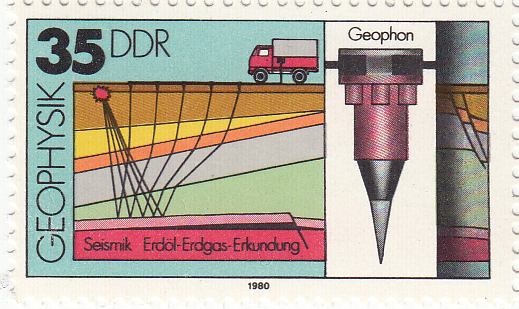
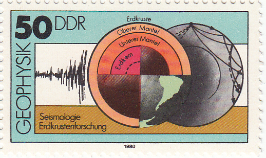
← The 50 pfennig stamp in the series of four shows not an instrument, but the method of deep-earth seismology. Earthquakes' seismic traces, left-most, are the basic pieces of data. Seismologists analyse the paths of these signals through the earth's crust (Erdkruste), mantle (Mantel) and core (Erdkern), right-most. The result is a model of the earth's deep interior, centre. Erdkrustenforschung translates as earth crust surveying. The actual size of the stamp is 43 × 26 mm.

To petroleum geophysicists and interpreters, global seismology may seem like a poor sibling of reflection seismology. But the science began with earthquake monitoring, which is centuries old. Earthquakes are the natural source of seismic energy for global seismological measurements; Zoeppritz wrote his equations about earthquake waves. (I don't know, but I can imagine seismologists feeling a guilty pang of anticipation when hearing of even quite deadly earthquakes.)

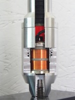
The M9.2 Sumatra-Andaman earthquake of 2004 lasted for an incredible 500 seconds—compared to a few seconds or tens of seconds for most earthquakes felt by humans. Giant events like this are rare (once a decade), and especially valuable because of the broad band of frequencies and very high amplitudes they generate. This allows high-fidelity detection by precision digital instruments like the Streckeisen STS-1 seismometer, positioned all over the world in networks like the United States' Global Seismographic Network, and the meta-network coordinated by the Federation of Digital Seismograph Networks, or FDSN. And these wavefields need global receiver arrays. 

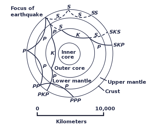
The basic structure of the earth was famously elucidated decades ago by these patterns of wave reflection and refraction through the earth's fundamentally concentric spheres of the solid inner core, liquid outer core, viscous mantle, and solid crust. For example, the apparent inability of the outer core to support S-waves is the primary evidence for its interpretation as a liquid. Today, global seismologists are more concerned with the finer points of this structure, and eking more resolution out of the intrinsically cryptic filter that is the earth. Sound familiar? What we do in exploration seismology is just a high-resolution, narrow-band, controlled-source extension of these methods. 

The last chat chart

The 1IWRP technical program was closed with a one-hour brainstorming session; an attempt to capture the main issues and ideas moving forward. This was great stuff, and I was invited to jot down the bombardment of shout-outs from the crowd.   

Admittedly, no list is fully comprehensive, and this flip chart is almost laughable in its ruggedness. However, I think it represents the diversity in this crowd and the relevant issues that people will be working on in the future. The main points were:

• Creating a common model and data sharing

• The future of digital rock physics

• Dealing with upscaling and scale dependant measurements

• The use of rock physics for improving sub-salt AVO analyses

• Strengthening the connection between rock physics and geomechanical applications

• Improvements for the next workshop at the University of South Hampton, in 2013.

I have scribed this into a more legible form, and put some expanded commentary on AgileWiki if you want to read more about these points. 

Do you disagree with anything on this list? Have we missed something?

More 1IWRP highlights

As I reported on Wednesday, I've been at 1IWRP, a workshop on rock physics in the petroleum industry. Topics ranged from lab core studies to 3D digital scanners, and from seismic attenuation and dispersion to shales and anisotropy. Rock physics truly crosses a lot of subject areas.

Here are a few of the many great talks that really stood out for me:

Mark Chapman from the University of Edinburgh, submitted a new formulation for frequency dependant AVO analysis. He suggested that if a proper rock physics model of the rock is described, frequency can be decomposed from seismic gathers for improved reservoir characterization. Some folks in the crowd warned that the utility of this work might be limited to select cases with a full band impedance change, but his method appears to be a step beyond the traditional AVO workflow.

Arthur Cheng from Halliburton talked about modeling techniques to estimate anisotropic parameters from borehole measurements. He descibed the state of the art in acoustic logging tools, and used a ray-tracing VSP forward model to show a significant smear of reflection points through an anisotropic earth layer. He touched on the importance of close interaction between service companies and end users, especially those working in complex environments. In particular: service companies have a good understanding of data precision and accuracy, but it's usually not adequately transfered to the interpreter.

Colin Sayers from Schlumberger presented several talks, but I really enjoyed what he had to say about sonic and seismic anisotropy and how it is relevant to characterizing shale gas reservoirs. Fracture propagation depends on the 3D stress state in the rock: hard to capture with a 1D earth model. He showed an example of how hydraulic fracture behaviour could be more accurately predicted by incorporating anisotropic stress dependant elastic properties. I hope this insight permeates throughout the engineering community. 

Rob Lander from Geocosm showed some fresh-out-of-the-oven simulations of coupled diagenesis and rock physics models for predicting reservoir properties away from wells. His company's workflow has a basis in petrography, integrating cathodluminescence microscopy and diagenetic modeling. Really inspiring and integrated stuff. I submit to you that this presentation would be equally enjoyed at a meeting of AAPG, SPE, SPWLA, SEG, or SCA — that's not something that you can say about every talk. 

← Every break heralded a new discussion. The delegates were very actively engaged. 

Today, I am going on a field trip to the Niobrara Shale Quarry. After four days indoors, I'm looking forward to getting outside and hammering some rocks! 

Digital rocks and accountability

There were three main sessions at the first day of the First International Workshop on Rock Physics, 1IWRP. Experimental methods, Digital rock physics, and Methods in rock physics, a softer, more philosophical session on perspectives in the lab and in the field. There have been several sessions of discussion too, occurring after every five presentations or so, which has been a refreshing addition to the program. I am looking for talks that will change the way we do things and two talks really stood out for me. 

Mark Knackstedt from Digitalcore in Australia, gave a visually stunning presentation on the state of the art in digital rock physics. You can browse Digitalcore's website and and view some of the animations that he showed. A few members of the crowd were skeptical about the nuances of characterizing microcracks and grain contacts near or below the resolution limits, as these tiny elements have a dominating role on a material's effective properties.  

In my opinion, in order to get beyond 3D visualizations, and the computational aspect of pixel counting, digital rock physicists need to integrate with petrophysicists to calibrate with logging tools. One exciting opportunity is deducing a link between laboratory and borehole-based NMR measurements for pore space and fluid characterization. 

In an inspired and slightly offbeat talk, Bill Murphy 3 from e4sciences challenged the community to make the profession better by increasing accountability. Being accountable means acknowledging what you know and what you don't know. He offered Atul Gawande's surgical writings as a model for all imperfect sciences. Instead of occupying a continuum from easy to hard, rock physics problems span a ternary space from simple to complicated to complex. Simple is something that can be described by a recipe or a definite measurement, complicated is like going to the moon, and complex is like raising a child, where there's an element of unpredictability. Part of our profession should be recognizing where our problems fall in this ternary space, and that should drive how we deal with these problems.

He also explained that ours is a science full of paradoxes:

• Taking more measurements means that we need to make more hypotheses, not fewer
• Ubiquitous uncertainty must be met with increased precision and rigor
• Acknowledging errors is essential for professional and scientific accountability

The next time you are working on a problem, why not estimate where it plots in this ternary space? It's likely to contain some combination of all three, and it might evolve as the project progresses. And ask your colleagues where they would place the same problem—it might surprise you. 

Why petrophysics is hard

Earlier this week we published our fourth cheatsheet, this time for well log analysis or petrophysics. (Have you seen our other cheatsheets?) Why did we think this was a subject tricky enough to need a cheatsheet in the back of your notebook? I think there are at least three things which make the interpretation of log data difficult:

Most of the tools do not directly measure properties we are interested in. For example, the radioactivity of the rocks is not important to us, but it does make a reliable clay and organic matter proxy, because these substances tend to have more uranium and other radioactive elements in them. Almost all of the logs are just proxies for the data we really need. 

We only see the rocks through the filter of the method. Even if we could perfectly derive apparent reservoir properties from the logs, there are lots of reasons why they might be less than accurate. For example, the drilling fluid (usually some sort of brine- or oil-based suspension of mud) tends to invade the rocks, especially the more permeable formations, the very ones we are interested in. The drilling fluid can also interfere with some tools, depending on its composition: barite absorbs gamma-rays, for example. 

The field is infested with jargon and historical baggage. Since Conrad and Marcel Schlumberger invented the technique almost 100 years ago, thousands of new tools and new methods have been invented. Every tool and log has its own name, method (usually proprietary these days) and idiosyncracies, making for a bewildering, intimidating even, menagerie. Worse still, lots of modern tools collect multi-dimensional data: for example, sonic spectra on multiple axes, magnetic resonance T2 distributions, dynamically-scaled image logs. 

We drew from several sources to build our cheatsheet. We drew partly from our own experience, but also relied on input from some petrophysical specialists: Neil Watson of Atlantic Petrophysics, Andrea Creemer of Corridor Resources, and Ross Crain of Spectrum 2000. We also consulted the following references, synthesizing liberally where they disagreed (quite often, given the range of vintages of these works).

• Schlumberger (1991), Log Interpretation Principles/Applications, Schlumberger Educational Services, Houston
• Rider, M (1991), The Geological Interpretation of Well Logs, Whittles Publishing, Caithness
• Crain, ER (2011). Crain's Petrophysical Handbook.
• Schlumberger's online documentation
• Halliburton's online documentation
• Paul Glover's course notes 

Despite referring to some of the best sources in the industry, we hereby assert that all errors are attributable to us, not our sources. If you find errors, please let us know. Get in touch on Twitter, use the contact form, or leave a comment.

Part of Viking's Provost A4-23 in 36-6, in Alberta, Canada.

Petrophysics cheatsheet

Geophysical logging is magic. After drilling, a set of high-tech sensors is lowered to the bottom of the hole on a cable, then slowly pulled up collecting data as it goes. A sort of geological endoscope, the tool string can measure manifold characteristics of the rocks the drillbit has penetrated: temperature, density, radioactivity, acoustic properties, electrical properties, fluid content, porosity, to name a few. The result is a set of well logs or wireline logs.

The trouble is there are a lot of different logs, each with its own idiosyncracies. The tools have different spatial resolutions, for example, and are used for different geological interpretations. Most exploration and production companies have specialists, called petrophysicists, to interpret logs. But these individuals are sometimes (usually, in my experience) thinly spread, and besides all geologists and geophysicists are sometimes faced with interpreting logs alone.

We wanted to make something to help the non-specialist. Like our previous efforts, our new cheatsheet is a small contribution, but we hope that you will want to stick it into the back of your notebook. We have simplified things quite a bit: almost every single entry in this table needs a lengthy footnote. But we're confident we're giving you the 80% solution. Or 70% anyway. 

Please let us know if and how you use this. We love hearing from our users, especially if you have enhancements or comments about usability. You can use the contact form, or leave a comment here. 

Update on 2011-07-27 13:25 by Matt Hall

Don't miss the follow-up to this post, from Wednesday 27 July, in which we explain why we thought we needed to build this cheatsheet.

And if you like this, please don't miss our other cheatsheets!

Geophysical stamps 3: Geophone

Back in May I bought some stamps on eBay. I'm not really a stamp collector, but when I saw these in all their geophysical glory, I couldn't resist them. They are East German stamps from 1980, and they are unusual because they aren't schematic illustrations so much as precise, technical drawings. I have already written about the the gravimeter and the sonic tool stamps; today I thought I'd tell a bit about the most basic seismic sensor, the geophone.

← The 35 pfennig stamp in the series of four shows a surface geophone, with a schematic cross-section and cartoon of the seismic acquisition process, complete with ray-paths and a recording truck. Erdöl and Erdgas are oil and gas, Erkundung translates as surveying or exploration. The actual size of the stamp is 43 × 26 mm.

There are four basic types of seismic sensor (sometimes generically referred to as receivers in exploration geophysics):

Seismometers — precision instruments not used in exploration seismology because they are usually quite bulky and require careful set-up and calibration. [Most modern models] are accelerometers, much like relative gravimeters, measuring ground acceleration from the force on a proof mass. Seismometers can detect frequencies in a very broad band, on the order of 0.001 Hz to 500 Hz: that's 19 octaves!

Geophones — are small, cheap, and intended for rapid deployment in large numbers. The one illustrated on the stamp, like the modern cut-away example shown here, would be about 4 × 20 cm, with a total mass of about 400 g. The design has barely changed in decades. The mean-looking spike is to try to ensure good contact with the ground (coupling). A frame-mounted magnet is surrounded by a proof mass affixed to a copper coil. This analog instrument measures particle [velocity], not acceleration, as the differential motion induces a current in the coil. Because of the small proof mass, the lower practical frequency limit is usually only about 6 Hz, the upper about 250 Hz (5 octaves). Geophones are used on land, and on the sea-floor. If repeatability over time is important, as with a time-lapse survey, phones like this may be buried in the ground and cemented in place.

Hydrophones — as the name suggests, are for deployment in the water column. Naturally, there is a lot of non-seismic motion in water, so measuring displacement will not do. Instead, hydrophones contain two piezoelectric components, which generates a current when deformed by pressure, and use cunning physics to mute spurious, non-seismic pressure changes. Hydrophones are usually towed in streamers behind a boat. They have a similar response band to geophones.

MEMS accelerometers — exactly like the accelerometer chip in your laptop or cellphone, these tiny mechanical systems can be housed in a robust casing and used to record seismic waves. Response frequencies range from 4–1000 Hz (8 octaves; theoretically they will measure down to 0 Hz, or DC in geophysish, but not in my experience). These are sometimes referred to as digital receivers, but they are really micro-analog devices with built-in digital conversion. 

I think the geophone is the single most important remote sensing device in geoscience. Is that justified hyperbole? A couple of recent stories from Scotland and Spain have highlighted the incredible clarity of seismic images, which can be awe-inspiring as well as scientifically and economically important.

Next time I'll look at the 50 pfennig stamp, which depicts deep seismic tomography. 

Update on 2011-07-17 11:03 by Matt Hall

Thank you to @hypocentre for the enlightening comments about these instruments. I changed some details in the text (in the square brackets) to reflect them. 

In researching this question, I came across Michael Hons' MSc thesis. Michael was part of the CREWES project at the University of Calgary, and I've seen him talk a coupe of times—I should have looked at it before! At the beginning of his dissertation, he gives a nice comparison of geophone (i.e. coil) and MEMS physics. There was one surprise (for me): MEMS accelerometers actually measure displacement, but because operational frequencies are so far below the resonant frequencies of the tiny proof mass, displacement is conveniently proportional to, and only instigated by, acceleration. So under normal circumstances, they are de facto accelerometers. 

Hons' thesis, Seismic sensing: Comparison of geophones and accelerometers using laboratory and field data, goes on to give a full comparison of geophones and MEMS and is well worth looking at if you deal with these instruments.

Building Tune*

Last Friday, I wrote a post on tuning effects in seismic, which serves as the motivation behind our latest app for Android™ devices, Tune*. I have done technical and scientific computing in the past, but I am a newcomer to 'consumer' software programming, so like Matt in a previous post about the back of the digital envelope, I thought I would share some of my experiences trying to put geo-computing on a mobile, tactile, always-handy platform like a phone.

Google's App Inventor tool has two parts: the interface designer and the blocks editor. Programming with the blocks involves defining and assembling a series of procedures and variables that respond to the user interface. I made very little progress doing the introductory demos online, and only made real progress when I programmed the tuning equation itself—the science. The equation only accounts for about 10% of the blocks. But the logic, control elements, and defaults that (I hope) result in a pleasant design and user experience, take up the remainder of the work. This supporting architecture, enabling someone else to pick it up and use it, is where most of the sweat and tears go. I must admit, I found it an intimidating mindset to design for somebody else, but perhaps being a novice means I can think more like a user? 

This screenshot shows the blocks that build the tuning equation I showed in last week's post. It makes a text block out of an equation with variables, and the result is passed to a graph to be plotted. We are making text because the plot is actually built by Google's Charts API, which is called by passing this equation for the tuning curve in a long URL. 

Upcoming versions of this app will include handling the 3-layer case, whereby the acoustic properties above and below the wedge can be different. In the future, I would like to incorporate a third dimension into the wedge space, so that the acoustic properties or wavelet can vary in the third dimension, so that seismic response and sensitivity can be tested dynamically.

Even though the Ricker wavelet is the most commonly used, I am working on extending this to include other wavelets like Klauder, Ormsby, and Butterworth filters. I would like build a wavelet toolbox where any type of wavelet can be defined based on frequency and phase spectra. 

Please let me know if you have had a chance to play with this app and if there are other features you would like to see. You can read more about the science in this app on the wiki, or get it from the Android Market. At the risk (and fun) of nakedly exposing my lack of programming prowess to the world, I have put a copy of the package on the DOWNLOAD page, so you can grab Tune.zip, load it into App Inventor and check it out for yourself. It's a little messy; I am learning more elegant and parsimonious ways to build these blocks. But hey, it works!