All the time freaks

Thursday was our last day at the SEG Annual Meeting. Evan and I took in the Recent developments in time-frequency analysis workshop, organized by Mirko van der Baan, Sergey Fomel, and Jean-Baptiste Tary (Vienna). The workshop came out of an excellent paper I reviewed this summer, which was published online a couple of weeks ago:

Tary, JB, RH Herrera, J Han, and M van der Baan (2014), Spectral estimation—What is new? What is next?, Rev. Geophys. 52. doi:10.1002/2014RG000461.

The paper compares the results of several time–frequency transforms on a suite of 'benchmark' signals. The idea of the workshop was to invite further investigation or other transforms. The organizers did a nice job of inviting contributors with diverse interests and backgrounds. The following people gave talks, several of them sharing their code (*):

• John Castagna (Lumina) with a review of the applications of spectral decomposition for seismic analysis.
• Steven Lin (NCU, Taiwan) on empirical methods and the Hilbert–Huang transform.
• Hau-Tieng Wu (Toronto) on the application of transforms to monitoring respiratory patterns in animals.*
• Marcílio Matos (SISMO) gave an entertaining, talk about various aspects of the problem.
• Haizhou Yang (Standford) on synchrosqueezing transforms applied to problems in anatomy.*
• Sergey Fomel (UT Austin) on Prony's method... and how things don't always work out.*
• Me, talking about the fidelity of time–frequency transforms, and some 'unsolved problems' (for me).*
• Mirko van der Baan (Alberta) on the results from the Tary et al. paper.

Some interesting discussion came up in the two or three unstructured parts of the session, organized as mini-panel discussions with groups of authors. Indeed, it felt like the session could have lasted longer, because I don't think we got very close to resolving anything. Some of the points I took away from the discussion:

• My observation: there is no existing survey of the performance of spectral decomposition (or AVO) — these would be great risking tools.
• Castagna's assertion: there is no model that predicts the low-frequency 'shadow' effect (confusingly it's a bright thing, not a shadow).
• There is no agreement on whether the so-called 'Gabor limit' of time–frequency localization is a lower-bound on spectral decomposition. I will write more about this in the coming weeks.
• Should we even be attempting to use reassignment, or other 'sharpening' tools, on broadband signals? To put it another way: does instantaneous frequency mean anything in seismic signals?
• What statistical measures might help us understand the amount of reassignment, or the precision of time–frequency decompositions in general?

The fidelity of time–frequency transforms

My own talk was one of the hardest I've ever done, mainly because I don't think about these problems very often. I'm not much of a mathematician, so when I do think about them, I tend to have more questions than insights, so I made my talk into a series of questions for the audience. I'm not sure I got much closer to any answers, but I have a better idea of my questions now... which is a kind of progress I suppose.

Here's my talk (latest slides — GitHub repo). Comments and feedback are, as always, welcome.

Big imaging, little imaging, and telescopes

I caught three lovely talks at the special session yesterday afternoon, Recent Advances and the Road Ahead. Here are my notes...

The neglected workhorse

If you were to count up all the presentations at this convention on seismic migration, only 6% of them are on time migration. Even though it is the workhorse of seismic data processing, it is the most neglected topic in migration. It's old technology, it's a commodity. Who needs to do research on time migration anymore? Sergey does.

Speaking as an academic, Fomel said, "we are used to the idea that most of our ideas are ignored by industry," even though many transformative ideas in the industry can be traced back to academics. He noted that it takes at least 5 years to get traction, and the 5 years are up for his time migration ideas, "and I'm starting to lose hope". Here's five things you probably didn't know about time migration:

• Time migration does not need travel times.
• Time migration does not need velocity analysis.
• Single offsets can be used to determine velocities.
• Time migration does need approximations, but the approximation can be made increasingly accurate.
• Time migration distorts images, but the distortion can be removed with regularized inversion.

It was joy to listen to Sergey describe these observations through what he called beautiful equations: "the beautiful part about this equation is that it has no parameters", or "the beauty of this equation is that is does not contain velocity", an so on. Mad respect.

Seismic adaptive optics

Alongside seismic multiples, poor illumination, and bandwidth limitations, John Etgen (BP) submitted that, in complex overburden, velocity is the number one problem for seismic imaging. Correct velocity model equals acceptable image. His (perhaps controversial) point was that when velocities are complex, multiples, no matter how severe, are second order thorns in the side of the seismic imager. "It's the thing that's killing us, and that's the frontier." He also posited that full waveform inversion may not save us after all, and image gather analysis looks even less promising.

While FWI looks to catch the wavefield and look at it in the space of the data, migration looks to catch the wavefield and look at it at the image point itself. He elegantly explained these two paradigms, and suggested that both may be flawed.

John urged, "We need things other than what we are working on", and shared his insights from another field. In ground-based optical astronomy, for example, when the image of a star is be distorted by turbulence in our atmosphere, astromoners numerically warp the curvature of the lens to correct for rapid variations in phase of the incoming wavefront. The lenses we use for seismic focusing, velocities, can be tweaked just the same by looking at the wavefield part of the way through its propagation. He quoted Jon Claerbout:

If you want to understand how a horse runs, you gotta run along with it.

Big imaging, little imaging, and combination of the two

There's a number of ways one could summarize what petroleum seismologists do. But hearing (CGG researcher) Sam Gray's talk yesterday was a bit of an awakening. His talk was a remark on the notion of big imaging vs little imaging, and the need for convergence.

Big imaging is the structural stuff. Structural migration, stratigraphic imaging, wide-azimuth acquisition, and so on. It includes the hardware and compute innovations of broadband, blended sources, deblending processing, anisotropic imaging, and the beginnings of viscoacoustic reverse-time migration. 

Little imaging is inversion. It's reservoir characterization. It's AVO and beyond. Azimuthal velocities (fast and slow directions) hint at fracture orientations, azimuthal amplitudes hint even more subtly at fracture compliance.

Big imaging is hard because it's computationally expensive, and velocities are unknown. Little imaging is hard because features like fractures, faults and pores are at the centimetre scale, but on land we lay out inlines and crossline hundreds of metres apart, and use signals that carry only a few bits of information from an area the size of a football field.

What we've been doing with imaging is what he called a separated workflow. We use gathers to make big images. We use gathers to make rock properties, but seldom do they meet. How often have you tested to see if the rock properties the little are explain the wiggles in the big? Our work needs to be such a cycle, if we want our relevance and impact to improve.

The figures are copyright of the authors of SEG, and used in accordance with SEG's permission guidelines.

October linkfest

The linkfest has come early this month, to accommodate the blogging blitz that always accompanies the SEG Annual Meeting. If you're looking forward to hearing all about it, you can make sure you don't miss a thing by getting our posts in your email inbox. Guaranteed no spam, only bacn. If you're reading this on the website, just use the box on the right →

---

Open geoscience goodness

I've been alerted to a few new things in the open geoscience category in the last few days:

• Dave Hale released his cool-looking fault detection code
• Wayne Mogg released some OpendTect plugins for AVO, filtering, and time-frequency decomposition
• Joel Gehman and others at U of A and McGill have built WellWiki, a wiki... for wells!
• Jon Claerbout, Stanford legend, has released his latest book with Sergey Formel, Austin legend: Geophysical Image Estimation by Example. As you'd expect, it's brilliant, and better still: the code is available. Amazing resource.

And there's one more resource I will mention, but it's not free as in speech, only free as in beer — Petroacoustics: A Tool for Applied Seismics, by Patrick Rasolofosaon and Bernard Zinszner. So it's nice because you can read it, but not that useful because the terms of use are quite stringent. Hat tip to Chris Liner.

So what's the diff if things are truly open or not? Well, here's an example of the good things that happen with open science: near-real-time post-publication peer review and rapid research: How massive was Dreadnoughtus?

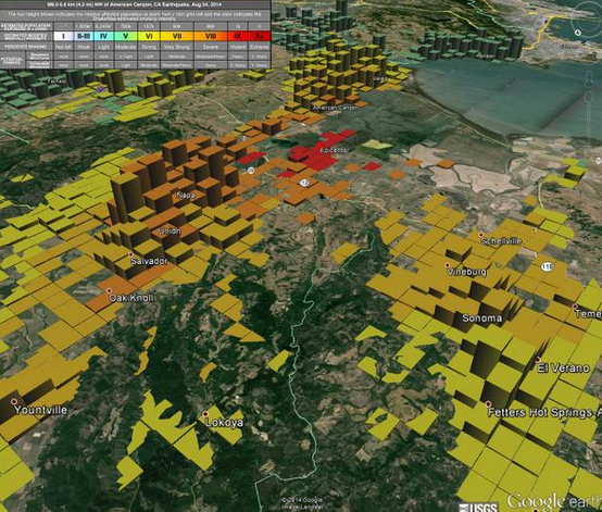
Technology and geoscience

Open data sharing has great potential in earthquake sensing, as there are many more people with smartphones than there are seismometers. The USGS shake map (right) is of course completely perceptual, but builds in real time. And Jawbone, makers of the UP activity tracker, were able to sense sleep interruption (in their proprietary data): the first passive human-digital sensors?

We love all things at the intersection of the web and computation... so Wolfram Alpha's new "Tweet a program" bot is pretty cool. I asked it:

GeoListPlot[GeoEntities[=[Atlantic Ocean], "Volcano"]]

And I got back a map!

This might be the coolest piece of image processing I've ever seen. Recovering sound from silent video images:

Actually, these time-frequency decompositions [PDF] of frack jobs are just as cool (Tary et al., 2014, Journal of Geophysical Research: Solid Earth 119 (2), 1295-1315). These deserve a post of their own some time.

It turns out we can recover signals from all sorts of unexpected places. There were hardly any seismic sensors around when Krakatoa exploded in 1883. But there were plenty of barometers, and those recorded the pressure wave as it circled the earth — four times! Here's an animation from the event.

It's hard to keep up with all the footage from volcanic eruptions lately. But this one has an acoustic angle: watch for the shockwave and the resulting spontaneous condensation in the air. Nonlinear waves are fascinating because the wave equation and other things we take for granted, like the superposition principle and the speed of sound, no longer apply.

Discussion and collaboration

Our community has a way to go before we ask questions and help each other as readily as, say, programmers do, but there's enough activity out there to give hope. My recent posts (one and two) about data (mis)management sparked a great discussion both here on the blog and on LinkedIn. There was also some epic discussion — well, an argument — about the Lusi post, as it transpired that the story was more complicated that I originally suggested (it always is!). Anyway, it's the first debate I've seen on the web about a sonic log. And there continues to be promising engagement on the Earth Science Stack Exchange. It needs more applied science questions, and really just more people. Maybe you have a question to ask...?

Géophysiciens avec des ordinateurs

Don't forget there's the hackathon next weekend! If you're in Denver, free come along and soak up the geeky rays. If you're around on the afternoon of Sunday 26 October, then drop by for the demos and prizes, and a local brew, at about 4 pm. It's all happening at Thrive, 1835 Blake Street, a few blocks north of the convention centre. We'll all be heading to the SEG Icebreaker right afterwards. It's free, and the doors will be open.

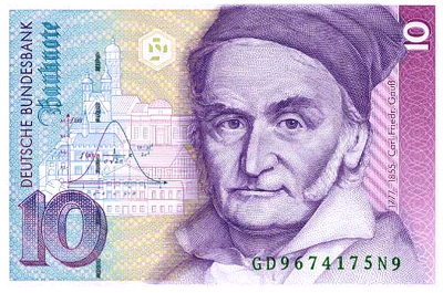
Great geophysicists #12: Gauss

Carl Friedrich Gauss was born on 30 April 1777 in Braunschweig (Brunswick), and died at the age of 77 on 23 February 1855 in Göttingen. He was a mathematician, you've probably heard of him; he even has his own Linnean handle: Princeps mathematicorum, or Prince of mathematicians (I assume it's the royal kind, not the Purple Rain kind — ba dum tss).

Gauss's parents were poor, working class folk. I wonder what they made of their child prodigy, who allegedly once stunned his teachers by summing the integers up to 100 in seconds? At about 16, he was quite a clever-clogs, rediscovering Bode's law, the binomial theorem, and the prime number theorem. Ridiculous.

His only imperfection was that he was too much of a perfectionist. His motto was pauca sed matura, meaning "few, but ripe". It's understandable how someone so bright might not feel much need to share his work, but historian Eric Temple Bell reckoned that if Gauss had published his work regularly, he would have advanced mathematics by fifty years.

He was only 6 when Euler died, but surely knew his work. Euler is the only other person who made comparably broad contributions to what we now call the exploration geophysics toolbox, and applied physics in general. Here are a few: 

• He proved the fundamental theorems of algebra and arithmetic. No big deal.
• He formulated the Gaussian function — which of course crops up everywhere, especially in geostatistics. The Ricker wavelet is a pulse with frequencies distributed in a Gaussian.
• The gauss is the cgs unit of magnetic flux density, thanks to his work on the flux theorem, one of Maxwell's equations.
• He discovered the Cauchy integral theorem for contour integrals but did not publish it.
• The 'second' or 'total' curvature — a coordinate-system-independent measure of spatial curvedness — is named after him.
• He made discoveries in non-Euclidean geometry, but did not publish them.

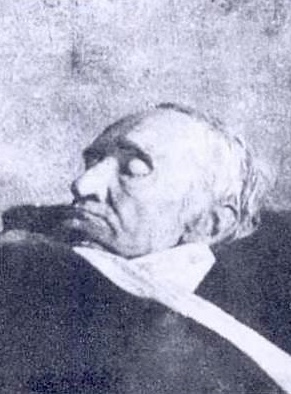
Excitingly, Gauss is the first great geophysicist we've covered in this series to have been photographed (right). Unfortunately, he was already dead. But what an amazing thing, to peer back through time almost 160 years.

Next time: Augustin-Jean Fresnel, a pioneer of wave theory.

The hackathon is coming

The Geophysics Hackathon is one month away! Signing up is not mandatory — you can show up on the day if you like — but it does help with the planning. It's 100% free, and I guarantee you'll enjoy yourself. You'll also learn tons about geophysics and about building software. Deets: Thrive, Denver, 8 am, 25–26 October. Bring a laptop.

Need more? Here's all the info you could ask for. Even more? Ask by email or in the comments. 

Send your project ideas

The theme this year is RESOLUTION. Participants are encouraged to post projects to hackathon.io ahead of time — especially if you want to recruit others to help. And even if you're not coming to the event, we'd love to hear your project ideas. Here are some of the proto-ideas we have so far: 

• Compute likely spatial and temporal resolution from some basic acquisition info: source, design, etc.
• Do the same but from information from the stack: trace spacing, apparent bandwidth, etc.
• Find and connect literature about seismic and log resolution using online bibliographic data.
• What does the seismic spectrum look like, given STFT limitations, or Gabor uncertainty?

If you have a bright idea, get in touch by email or in the comments. We'd love to hear from you.

Thank you to our sponsors

Three forward-thinking companies have joined us in making the hackathon as much a geophysics party as well as a scientific workshop (a real workshop). I think this industry may have trained us to take event sponsorship for granted, but it's easy to throw $5000 at the Marriott for Yet Another Coffee Break. Handing over money to a random little company in Nova Scotia to buy coffee, tacos, and cool swag for hungry geophysicists and programmers takes real guts! 

Please take a minute to check out our sponsors and reward them for supporting innovation in our community. 

Students: we are offering $250 bursaries to anyone looking for help with travel or accommodation. Just drop me a line with a project idea. If you know a student that might enjoy the event, please forwadrd this to them.

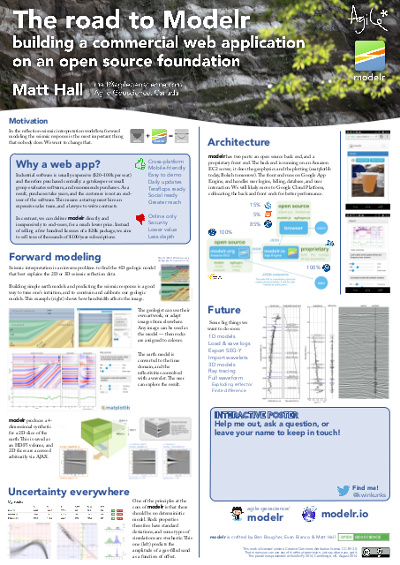
The road to Modelr: my EuroSciPy poster

At EuroSciPy recently, I gave a poster-ized version of the talk I did at SciPy. Unlike most of the other presentations at EuroSciPy, my poster didn't cover a lot of the science (which is well understood), or the code (which is esoteric).

Instead it focused on the advantages of spreading software via web applications, rather than only via source code, and on the challenges that we overcame — well, that we're still overcoming — to get our Modelr tool out there. I wanted other programmer-scientists to think about running some of their code as a web app for others to enjoy, but to be aware of the effort involved in doing this.

I've written before about my dislike of posters, though I'm told they are an important component at, say, the AGU Fall Meeting. I admit I do quite like the process of making them, and — on advice from Colin Purrington's useful page — I left a space on the poster for people to write comments or leave sticky notes. As a result, I heard about Docker, a lead I'll certainly follow up,

What's new in modelr

This wasn't part of the poster, but I might as well take the chance to let you know what we've updated recently:

• You can now add noise to models by specifying the signal:noise.
• Instead of automatic scaling, you can choose your own gain.
• The app now returns the elastic moduli of the rocks in the model.
• You can choose a spatial cross-section view or a space–offset–frequency view.

All of these features are now available to subscribers for only $9/month. Amazing value :)

Figshare

I've stored my poster on Figshare, a data storage site and part of Macmillan's Digital Science effort. What I love about Figshare, apart from the convenience of cloud-based storage and easy access for others, is that every item gets a digital object identifier or DOI. You've probably seen these on journal articles. They're a bit like other persistent and unique IDs for publications, such as ISBNs for books, but the idea is to provide more interactivity by making it easily linkable: you can get to any object with a DOI by prepending it with "http://dx.doi.org/".

Reference

Hall, M (2014). The road to modelr: building a commercial web app on an open source foundation. EuroSciPy, Cambridge, UK, August 29–30, 2014. Poster presentation. DOI:10.6084/m9.figshare.1151653

Julia in a nutshell

Julia is the most talked-about language in the scientific Python community. Well, OK, maybe second to Python... but only just. I noticed this at SciPy in July, and again at EuroSciPy last weekend.

As promised, here's my attempt to explain why scientists are so excited about it.

Why is everyone so interested in Julia?

At some high level, Julia seems to solve what Steven Johnson (MIT) described at EuroSciPy on Friday as 'the two-language problem'. It's also known as Outerhout's dichotomy. Basically, there are system languages (hard to use, fast), and scripting languages (easy to use, slow). Attempts to get the best of boths worlds have tended to result in a bit of a mess. Until Julia.

Really though, why?

Cheap speed. Computer scientists adore C because it's rigorous and fast. Scientists and web developers worship Python because it's forgiving and usually fast enough. But the trade-off has led to various cunning ploys to get the best of both worlds, e.g. PyPy and Cython. Julia is perhaps the cunningest ploy of all, achieving speeds that compare with C, but with readable code, dynamic typing, garbage collection, multiple dispatch, and some really cool tricks like Unicode variable names that you enter in pure LaTeX. And check out this function definition shorthand:

Why is Julia so fast?

Machines don't understand programming languages — the code written by humans has to be translated into machine language in a process called 'compiling'. There are three approaches:

• Compile ahead of time — e.g. Fortran, C, C++
• Compile just in time (often called JIT) — e.g. JavaScript, Julia
• Interpret — e.g. Python, MATLAB, Perl, Ruby

Compiling makes languages fast, because the executed code is tuned to the task (e.g. in terms of the types of variables it handles), and to the hardware it's running on. Indeed, it's only by building special code for, say, integers, that compiled languages achieve the speeds they do.

Julia is compiled, like C or Fortran, so it's fast. However, unlike C and Fortran, which are compiled before execution, Julia is compiled at runtime ('just in time' for execution). So it looks a little like an interpreted language: you can write a script, hit 'run' and it just works, just like you can with Python.

You can even see what the generated machine code looks like:

Don't worry, I can't read it either.

But how is it still dynamically typed?

Because the compiler can only build machine code for specific types — integers, floats, and so on — most compiled languages have static typing. The upshot of this is that the programmer has to declare the type of each variable, making the code rather brittle. Compared to dynamically typed languages like Python, in which any variable can be any type at any time, this makes coding a bit... tricky. (A computer scientist might say it's supposed to be tricky — you should know the type of everything — but we're just trying to get some science done.)

So how does Julia cope with dynamic typing and still compile everything before execution? This is the clever bit: Julia scans the instructions and compiles for the types it finds — a process called type inference — then makes the bytecode, and caches it. If you then call the same instructions but with a different type, Julia recompiles for that type, and caches the new bytecode in another location. Subsequent runs use the appropriate bytecode, with recompilation.

Metaprogramming

It gets better. By employing metaprogramming — on-the-fly code generation for special tasks — it's possible for Julia to be even faster than highly optimized Fortran code (right), in which metaprogramming is unpleasantly difficult. So, for example, in Fortran one might tolerate a relatively slow loop that can only be avoided with code generation tricks; in Julia the faster route is much easier. Here's Steven's example.

Interoperability and parallelism

It gets even better. Julia has been built with interoperability in mind, so calling C — or Python — from inside Julia is easy. Projects like Jupyter will only push this further, and I expect Julia to soon be the friendiest way to speed up that stubborn inner NumPy loop. And I'm told a lot of thoughtful design has gone into Julia's parallel processing libraries... I have never found an easy way into that world, so I hope it's true.

---

I'm not even close to being able to describe all the other cool things Julia, which is still a young language, can do. Much of it will only be of interest to 'real' programmers. In many ways, Julia seems to be 'Python for C programmers'.

If you're really interested, read Steven's slides and especially his notebooks. Better yet, just install Julia and IJulia, and play around. Here's another tutorial and a cheatsheet to get you started.

Highlights from EuroSciPy

In July, Agile reported from SciPy in Austin, Texas, one of several annual conferences for people writing scientific software in the Python programming language. I liked it so much I was hungry for more, so at the end of my recent trip to Europe I traveled to the city of Cambridge, UK, to participate in EuroSciPy.

The conference was quite a bit smaller than its US parent, but still offered 2 days of tutorials, 2 days of tech talks, and a day of sprints. It all took place in the impressive William Gates Building, just west of the beautiful late Medieval city centre, and just east of Schlumberger's cool-looking research centre. What follows are my highlights...

Okay you win, Julia

Steven Johnson, an applied mathematician at MIT, gave the keynote on the first morning. His focus was Julia, the current darling of the scientific computing community, and part of a new ecosystem of languages that seek to cooperate, not compete. I'd been sort of ignoring Julia, in the hope that it might go away and let me focus on Python, the world's most useful language, and JavaScript, the world's most useful pidgin... but I don't think scientists can ignore Julia much longer.

I started writing about what makes Julia so interesting, but it turned into another post — up next. Spoiler: it's speed. [Edit: Here is that post! Julia in a nutshell.]

Learning from astrophysics

The Astropy project is a truly inspiring community — in just 2 years it has synthesized a dozen or so disparate astronomy libraries into an increasingly coherent and robust toolbox for astronomers and atrophysicists. What does this mean?

• The software is well-tested and reliable.
• Datatypes and coordinate systems are rich and consistent.
• Documentation is useful and evenly distributed.
• There is a tangible project to rally developers and coordinate funding.

Geophysicists might even be interested in some of the components of Astropy and the related SunPy project, for example:

• astropy.units, just part of the ever-growing astropy library, as a unit conversion and quantity handler to compare with pint.
• sunpy datatypes map and spectra for types of data that need special methods.
• asv is a code-agnostic benchmarking library, a bit like freebench.

Speed dating for scientists

Much of my work is about connecting geoscientists in meaningful collaboration. There are several ways to achieve this, other than through project work: unsessions, wikis, hackathons, and so on. Now there's another way: speed dating.

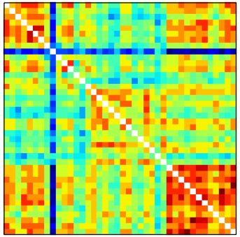
Okay, it doesn't quite get to the collaboration stage, but Vaggi and his co-authors shared an ingenious way to connect people and give their professional relationship the best chance of success (an amazing insight, a new algorithm, or some software). They asked everyone at a small 40-person conference to complete a questionnaire that asked, among other things, what they knew about, who they knew, and, crucially, what they wanted to know about. Then they applied graph theory to find the most desired new connections (the matrix shows the degree of similarity of interests, red is high), and gave the scientists five 10-minute 'dates' with scientists whose interests overlapped with theirs, and five more with scientists who knew about fields that were new to them. Brilliant! We have to try this at SEG.

Vaggi, F, T Schiavinotto, A Csikasz-Nagy, and R Carazo-Salas (2014). Mixing scientists at conferences using speed dating. Poster presentation at EuroSciPy, Cambridge, UK, August 2014. Code on GitHub.

Vaggi, F, T Schiavinotto, J Lawson, A Chessel, J Dodgson, M Geymonat, M Sato, R Carazo Salas, A Csikasz Nagy (2014). A network approach to mixing delegates at meetings. eLife, 3. DOI: 10.7554/eLife.02273

Other highlights

• sumatra to generate and keep track of simulations.
• vispy, an OpenGL-based visualization library, now has higher-level, more Pythonic components.
• Ian Osvald's IPython add-on for RAM usage.
• imageio for lightweight I/O of image files.
• nbagg backend for matplotlib version 1.4, bringin native (non-JS) interactivity.
• An on-the-fly kernel chooser in upcoming IPython 3 (currently in dev).

All in all, the technical program was a great couple of days, filled with the usual note-taking and hand-shaking. I had some good conversations around my poster on modelr. I got a quick tour of the University of Cambridge geophysics department (thanks to @lizzieday), which made me a little nostalgic for British academic institutions. A fun week!

Burrowing by burning

Most kind of mining are low-yield games. For example, the world's annual gold production would fit in a 55 m² room. But few mining operations I'm aware of are as low yield as the one that ran in Melle, France, from about 500 till 950 CE, producing silver for the Carolingian empire and Charlemagne's coins. I visited the site on Saturday.

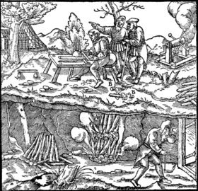
The tour made it clear just how hard humans had to work to bring about commerce and industry in the Middle Ages. For a start, of course they had no machines, just picks and shovels. But the Middle Jurassic limestone is silicic and very hard, so to weaken the rock they set fires against the face and thermally shocked the rock to bits. The technique, called fire-setting, was common in the Middle Ages, and was described in detail by Georgius Agricola in his book De Re Metallica (right; aside: the best translation of this book is by Herbert Hoover!). Apart from being stupefyingly dangerous, the method is slow: each fire got the miners about 4 cm further into the earth. Incredibly, they excavated about 20 km of galleries this way, all within a few metres of the surface.

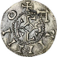
The fires were set against the walls and fuelled with wood, mostly beech. Recent experiments have found that one tonne of wood yielded about one tonne of rock. Since a tonne of rock yields 5 kg of galena, and this in turn yields 10 g of silver, we see that producing 1.1 tonnes of silver per year — enough for 640,000 deniers — was quite a feat!

There are several limits to such a resource intensive operation: wood, distance from face to works, maintenance, and willing human labour, not to mention the usual geological constraints. It is thought that, in the end, operations ended due to a shortage of wood.

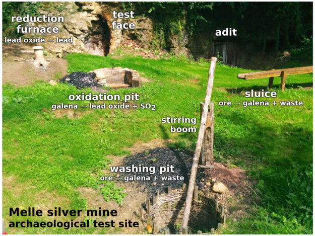
Several archaeologists visit the site regularly (here's one geospatial paper I found mentioning the site: Arles et al. 2013), and the evidence of their attempts to reproduce the primitive metallurgical methods were on display. Here's my attempt to label everything, based on what I could glean from the tour guide's rapid French:

The image of the denier coin is licensed CC-BY-SA by Wikipedia user Lequenne Gwendoline. 

At home with Leonardo

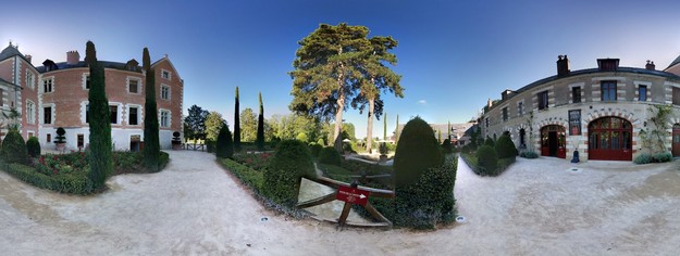
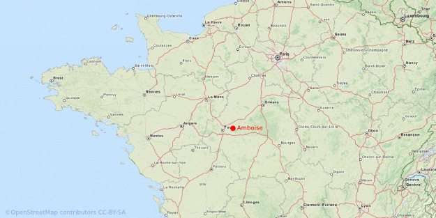
Well, OK, Leonardo da Vinci wasn't actually there, having been dead 495 years, but on Tuesday morning I visited the house at which he spent the last three years of his life. I say house, it's more of a mansion — the Château du Clos Lucé is a large 15th century manoir near the centre of the small market town of Amboise in the Loire valley of northern France. The town was once the royal seat of France, and the medieval grandeur still shows. 

Leonardo was invited to France by King Francis I in 1516. Da Vinci had already served the French governor of Milan, and was feeling squeezed from Rome by upstarts Rafael and Michelangelo. It's nice to imagine that Frank appreciated Leo's intellect and creativity — he sort of collected artists and writers — but let's face it, it was probably the Italian's remarkable capacity for dreaming up war machines, a skill he had honed in the service of mercenary and cardinal Cesare Borgia. Leonardo especially seemed to like guns; here are models of a machine gun and a tank, alongside more peaceful concoctions:

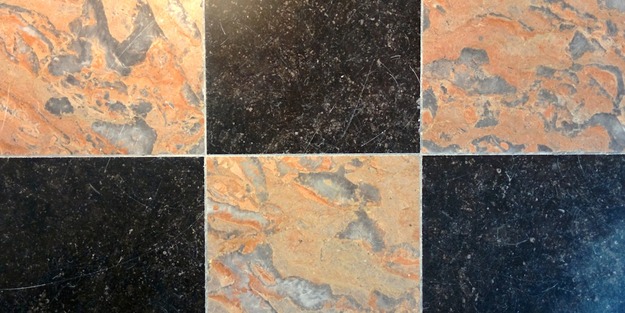
Inspired by José Carcione's assertion that Leonardo was a geophysicst, and plenty of references to fossils (even Palaeodictyon) in his notebooks, I scoured the place for signs of Leonardo dablling in geology or geophysics, but to no avail. The partly-restored Renaissance floor tiles did have some inspiring textures and lots of crinoid fossils... I wonder if he noticed them as he shuffled around?

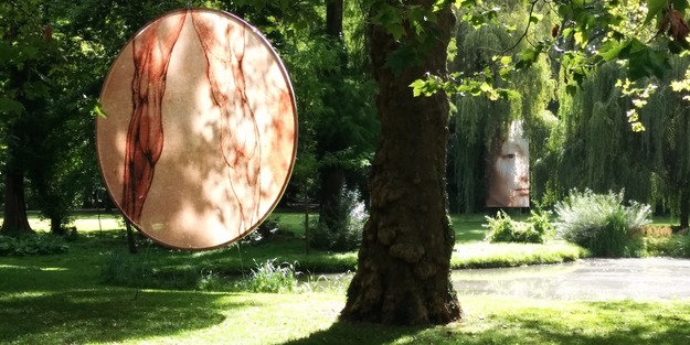
If you are ever in the area, I strongly recommend a visit. Even my kids (10, 6, and 4) enjoyed it, and it's close to some other worthy spots., specifically Chenonceau (for anyone) and Cheverny (for Tintin fans like me). The house, the numerous models, and the garden (below — complete with tasteful reproductions from Leonardo's works) were all terrific.

Check out José Carcione's two chapters about Leonardo and
his work in 52 Things You Should Know About Geophysics.
Download the chapter for free! [PDF, 3.8MB]