2013 retrospective

It's almost the end of the year, so we ask for your indulgence as we take our traditional look back at some of the better bits of the blog from 2013. If you have favourite subjects, we always like feedback!

Most visits

Amazingly, nothing we can write seems to be able to topple Shale vs tight, which is one of the firsts posts I wrote on this blog. Most of that traffic is coming from Google search, of course. I'd like to tell you how many visits the posts get, but web stats are fairly random — this year we'll have had either 60,000 or 245,000 visits, depending on who you believe — very precise data! Anyway, here are the rest...

• Interpreting spectral gamma-ray logs

• Well-tie workflow

• Expert culture is bad for you

Most comments

We got our 1000th blog comment at the end of September (thanks Matteo!). Admittedly some of them were us, but hey, we like arbitrary milestones as much as the next person. Here are the most commented-on posts of the year:

• Scientists not prospects, 16 comments — on dodgy marketing at conferences

• Geoscience, reservoir engineering, and code, 11 — on solving problems

• Must-read geophysics, 11 — on the top papers and books in geophysics

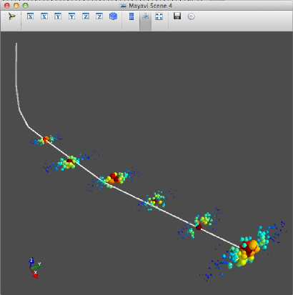
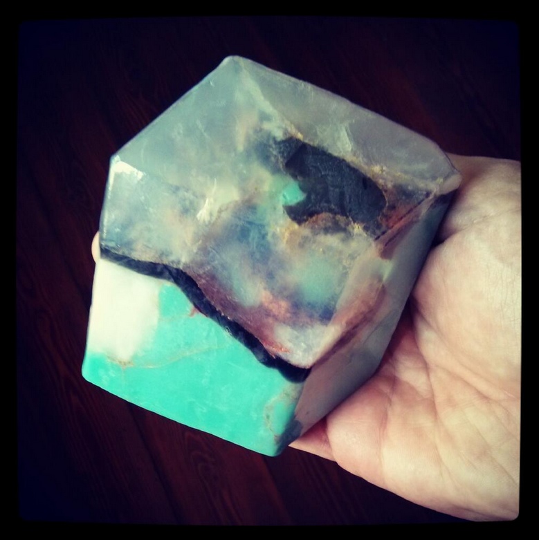
Hackathon skull

Proud moments

Some posts don't necessarily win a lot of readers or get many comments, but they mark events that were important to us. A sort of public record. Our big events in 2013 were...

• Unsolved Problems Unsession, Calgary in May

• Geophysics Hackthon, Houston in September

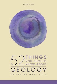
• The launch of the new book in November

Our favourites

Of course we have our personal favourite posts too — pieces that were especially fun to put together, or that took an unusual amount of craft and perspiration to finish (or more likely a sound beating with a blunt instrument).

Evan

• Backwards and forwards reasoning

• Expert culture is bad for you

• The calculus of geology

Matt

• Dream geoscience courses

• Filters that distort vision

• Colouring maps

I won't go into reader demographics as they've not changed much since last year. One thing is interesting, though not very surprising — about 15% of visitors are now reading on mobile devices, compared to 10% in 2012 and 7% in 2011. The technology shift is amazing: in 2011 we had exactly 94 visits from readers on tablets — now we get about 20 tablet visits every day, mostly from iPads.

It only remains for me to say Thank You to our wonderful community of readers. We appreciate every one of you, and love getting email and comments more than is probably healthy. The last 3 years have been huge fun, and we can't wait for 2014. If you celebrate Christmas may it be merry — and we wish you all the best for the new year.

To make up microseismic

I am not a proponent of making up fictitious data, but for the purposes of demonstrating technology, why not? This post is the third in a three-part follow-up from the private beta I did in Calgary a few weeks ago. You can check out the IPython Notebook version too. If you want more of this in person, sign up at the bottom or drop us a line. We want these examples to be easily readable, especially if you aren't a coder, so please let us know how we are doing.

Start by importing some packages that you'll need into the workspace,

%pylab inline

import numpy as np
from scipy.interpolate import splprep, splev
import matplotlib.pyplot as plt
import mayavi.mlab as mplt
from mpl_toolkits.mplot3d import Axes3D

Define a borehole path

We define the trajectory of a borehole, using a series of x, y, z points, and make each component of the borehole an array. If we had a real well, we load the numbers from the deviation survey just the same.

trajectory = np.array([[   0,   0,    0],
                       [   0,   0, -100],
                       [   0,   0, -200],
                       [   5,   0, -300],
                       [  10,  10, -400],
                       [  20,  20, -500],
                       [  40,  80, -650],
                       [ 160, 160, -700],
                       [ 600, 400, -800],
                       [1500, 960, -800]])
x = trajectory[:,0]
y = trajectory[:,1]
z = trajectory[:,2]

But since we want the borehole to be continuous and smoothly shaped, we can up-sample the borehole by finding the B-spline representation of the well path,

smoothness = 3.0
spline_order = 3
nest = -1 # estimate of number of knots needed (-1 = maximal)
knot_points, u = splprep([x,y,z], s=smoothness, k=spline_order, nest=-1)

# Evaluate spline, including interpolated points
x_int, y_int, z_int = splev(np.linspace(0, 1, 400), knot_points)

plt.gca(projection='3d')
plt.plot(x_int, y_int, z_int, color='grey', lw=3, alpha=0.75)
plt.show()

Define frac ports

Let's define a completion program so that our wellbore has 6 frac stages,

number_of_fracs = 6

and let's make it so that each one emanates from equally spaced frac ports spanning the bottom two-thirds of the well.

x_frac, y_frac, z_frac = splev(np.linspace(0.33, 1, number_of_fracs), knot_points)

Make a set of 3D axes, so we can plot the well path and the frac ports.

ax = plt.axes(projection='3d')
ax.plot(x_int, y_int, z_int, color='grey',
        lw=3, alpha=0.75)
ax.scatter(x_frac, y_frac, z_frac,
        s=100, c='grey')
plt.show()

Set a colour for each stage by cycling through red, green, and blue,

stage_color = []
for i in np.arange(number_of_fracs):
    color = (1.0, 0.1, 0.1)
    stage_color.append(np.roll(color, i))
stage_color = tuple(map(tuple, stage_color))

Define microseismic points

One approach is to create some dimensions for each frac stage and generate 100 points randomly within each zone. Each frac has an x half-length, y half-length, and z half-length. Let's also vary these randomly for each of the 6 stages. Define the dimensions for each stage:

frac_dims = []
half_extents = [500, 1000, 250]
for i in range(number_of_fracs):
    for j in range(len(half_extents)):
        dim = np.random.rand(3)[j] * half_extents[j]
        frac_dims.append(dim)  
frac_dims = np.reshape(frac_dims, (number_of_fracs, 3))

Plot microseismic point clouds with 100 points for each stage. The following code should launch a 3D viewer scene in its own window:

size_scalar = 100000
mplt.plot3d(x_int, y_int, z_int, tube_radius=10)
for i in range(number_of_fracs):
    x_cloud = frac_dims[i,0] * (np.random.rand(100) - 0.5)
    y_cloud = frac_dims[i,1] * (np.random.rand(100) - 0.5)
    z_cloud = frac_dims[i,2] * (np.random.rand(100) - 0.5)

    x_event = x_frac[i] + x_cloud
    y_event = y_frac[i] + y_cloud     
    z_event = z_frac[i] + z_cloud
    
    # Let's make the size of each point inversely proportional 
    # to the distance from the frac port
    size = size_scalar / ((x_cloud**2 + y_cloud**2 + z_cloud**2)**0.002)
    
    mplt.points3d(x_event, y_event, z_event, size, mode='sphere', colormap='jet')

You can swap out the last line in the code block above with mplt.points3d(x_event, y_event, z_event, size, mode='sphere', color=stage_color[i]) to colour each event by its corresponding stage.

A day of geocomputing

I will be in Calgary in the new year and running a one-day version of this new course. To start building your own tools, pick a date and sign up:

    

To make a wedge

We'll need a wavelet like the one we made last time. We could import it, if we've made one, but SciPy also has one so we can save ourselves the trouble. Remember to put %pylab inline at the top if using IPython notebook.

import numpy as np
from scipy.signal import ricker
import matplotlib.pyplot as plt

Now we need to make a physical earth model with three rock layers. In this example, let's make an acoustic impedance earth model. To keep it simple, let's define the earth model with two-way-travel time along the vertical axis (as opposed to depth). There are number of ways you could describe a wedge using math, and you could probably come up with a way that is better than mine. Here's a way:

nsamps, ntraces = [600, 500]
rock_names = ['shale 1', 'sand', 'shale 2']
rock_grid = np.zeros((n_samples, n_traces))

def make_wedge(n_samples, n_traces, layer_1_thickness, start_wedge, end_wedge):
    for j in np.arange(n_traces): 
        for i in np.arange(n_samples):      
            if i <= layer_1_thickness:      
                rock_grid[i][j] = 1    
            if i > layer_1_thickness:         
                rock_grid[i][j] = 3    
                if j >= start_wedge and i - layer_1_thickness < j-start_wedge: 
                    rock_grid[i][j] = 2
                    if j >= end_wedge and i > layer_1_thickness+(end_wedge-start_wedge):
                        rock_grid[i][j] = 3
    return rock_grid

Let's insert some numbers into our wedge function and make a particular geometry.

layer_1_thickness = 200
start_wedge = 50
end_wedge = 250
rock_grid = make_wedge(n_samples, n_traces, 
            layer_1_thickness, start_wedge, 
            end_wedge)

plt.imshow(rock_grid, cmap='copper_r')

Now we can give each layer in the wedge properties.

vp = np.array([3300., 3200., 3300.]) 
rho = np.array([2600., 2550., 2650.]) 
AI = vp*rho
AI = AI / 10e6 # re-scale (optional step)

Then assign values assign them accordingly to every sample in the rock model.

model = np.copy(rock_grid)
model[rock_grid == 1] = AI[0]
model[rock_grid == 2] = AI[1]
model[rock_grid == 3] = AI[2]

plt.imshow(model, cmap='Spectral')
plt.colorbar()
plt.title('Impedances')

Now we can compute the reflection coefficients. I have left out a plot of the reflection coefficients, but you can check it out in the full version in the nbviewer

upper = model[:-1][:]
lower = model[1:][:]
rc = (lower - upper) / (lower + upper)
maxrc = abs(np.amax(rc))

Now we make the wavelet interact with the model using convolution. The convolution function already exists in the SciPy signal library, so we can just import it.

from scipy.signal import convolve
def make_synth(f):
    synth = np.zeros((n_samples+len(t)-2, n_traces))
    wavelet = ricker(512, 1e3/(4.*f))
    wavelet = wavelet / max(wavelet)   # normalize
    for k in range(n_traces):
        synth[:,k] = convolve(rc[:,k], wavelet)
    synth = synth[ np.ceil(len(wavelet))/2 : -np.ceil(len(wavelet))/2, : ]
    return synth

Finally, we plot the results.

frequencies = array([5, 10, 15])
plt.figure(figsize = (15, 4))
for i in np.arange(len(frequencies)):
    this_plot = make_synth(frequencies[i])
    plt.subplot(1, len(frequencies), i+1)
    plt.imshow(this_plot, cmap='RdBu', vmax=maxrc, vmin=-maxrc, aspect=1)
    plt.title( '%d Hz wavelet' % freqs[i] )
    plt.grid()
    plt.axis('tight')
    
    # Add some labels
    for i, names in enumerate(rock_names):
        plt.text(400, 100+((end_wedge-start_wedge)*i+1), names,
                 fontsize=14, color='gray',
                 horizontalalignment='center',
                 verticalalignment='center')

 

That's it. As you can see, the marriage of building mathematical functions and plotting them can be a really powerful tool you can apply to almost any physical problem you happen to find yourself working on.

You can access the full version in the nbviewer. It has a few more figures than what is shown in this post.

A day of geocomputing

I will be in Calgary in the new year and running a one-day version of this new course. To start building your own tools, pick a date and sign up:

    

To plot a wavelet

As I mentioned last time, a good starting point for geophysical computing is to write a mathematical function describing a seismic pulse. The IPython Notebook is designed to be used seamlessly with Matplotlib, which is nice because we can throw our function on graph and see if we were right. When you start your own notebook, type

ipython notebook --pylab inline

We'll make use of a few functions within NumPy, a workhorse to do the computational heavy-lifting, and Matplotlib, a plotting library.

import numpy as np
import matplotlib.pyplot as plt

Next, we can write some code that defines a function called ricker. It computes a Ricker wavelet for a range of discrete time-values t and dominant frequencies, f:

def ricker(f, length=0.512, dt=0.001):
    t = np.linspace(-length/2, (length-dt)/2, length/dt)
    y = (1.-2.*(np.pi**2)*(f**2)*(t**2))*np.exp(-(np.pi**2)*(f**2)*(t**2))
    return t, y

Here the function needs 3 input parameters; frequency, f, the length of time over which we want it to be defined, and the sample rate of the signal, dt. Calling the function returns two arrays, the time axis t, and the value of the function, y.

To create a 5 Hz Ricker wavelet, assign the value of 5 to the variable f, and pass it into the function like so,

f = 5
t, y = ricker (f)

To plot the result,

plt.plot(t, y)

But with a few more commands, we can improve the cosmetics,

plt.figure(figsize=(7,4))
plt.plot( t, y, lw=2, color='black', alpha=0.5)
plt.fill_between(t, y, 0,  y > 0.0, interpolate=False, hold=True, color='blue', alpha = 0.5)
plt.fill_between(t, y, 0, y < 0.0, interpolate=False, hold=True, color='red', alpha = 0.5)

# Axes configuration and settings (optional)
plt.title('%d Hz Ricker wavelet' %f, fontsize = 16 )
plt.xlabel( 'two-way time (s)', fontsize = 14)
plt.ylabel('amplitude', fontsize = 14)
plt.ylim((-1.1,1.1))
plt.xlim((min(t),max(t)))
plt.grid()
plt.show()

Next up, we'll make this wavelet interact with a model of the earth using some math. Let me know if you get this up and running on your own.

Let's do it

It's short notice, but I'll be in Calgary again early in the new year, and I will be running a one-day version of this new course. To start building your own tools, pick a date and sign up:

    

Coding to tell stories

Last week, I was in Calgary on family business, but I took an afternoon to host a 'private beta' for a short course that I am creating for geoscience computing. I invited about twelve familiar faces who would be provide gentle and constuctive feedback. In the end, thirteen geophysicists turned up, seven of whom I hadn't met before. So much for familiarity.

I spent about two and half hours stepping through the basics of the Python programming language, which I consider essential material — getting set up with Python via Enthought Canopy, basic syntax, and so on. In the last hour of the afternoon, I steamed through a number of geoscientific examples to showcase exercises for this would-be course. 

Here are three that went over well. Next week, I'll reveal the code for making these images. I might even have a go at converting some of my teaching materials from IPython Notebook to HTML:

To plot a wavelet

The Ricker wavelet is a simple analytic function that is used throughout seismology. This curvaceous waveform is easily described by a single variable, the dominant frequency of its many contituents frequencies. Every geophysicist and their cat should know how to plot one: 

To make a wedge

Once you can build a wavelet, the next step is to make that wavelet interact with the earth. The convolution of the wavelet with this 3-layer impedance model yields a synthetic seismogram suitable for calibrating seismic signals to subtle stratigraphic geometries. Every interpreter should know how to build a wedge, with site-specific estimates of wavelet shape and impedance contrasts. Wedge models are important in all instances of dipping and truncated layers at or below the limit of seismic resolution. So basically they are useful all of the time. 

To make a 3D viewer

The capacity of Python to create stunning graphical displays with merely a few (thoughtful) lines of code seemed to resonate with people. But make no mistake, it is not easy to wade through the hundreds of function arguments to access this power and richness. It takes practice. It appears to me that practicing and training to search for and then read documentation, is the bridge that carries people from the mundane to the empowered.

This dry-run suggested to me that there are at least two markets for training here. One is a place for showing what's possible — "Here's what we can do, now let’s go and build it". The other, more arduous path is the coaching, support, and resources to motivate students through the hard graft that follows. The former is centered on problem solving, the latter is on problem finding, where the work and creativity and sweat is. 

Would you take this course? What would you want to learn? What problem would you bring to solve?

Update on 2013-12-10 13:17 by Evan Bianco

Update: the first follow-up post in this series is a code-based tutorial on how to plot a wavelet, and has an announcement about two 1-day events I will be holding in Calgary in the new year (January 10, and January 13, 2014).

Which brittleness index?

A few weeks ago I looked at the concept — or concepts — of brittleness. There turned out to be lots of ways of looking at it. We decided to call it a rock behaviour rather than a property. And we determined to look more closely at some different ways to define it. Here they are...

Some brittleness indices

There are lots of 'definitions' of brittleness in the literature. Several of them capture the relationship between compressive and tensile strength, σ_C and σ_T respectively. This is potentially useful, because we measure uniaxial compressive strength in the standard triaxial rig tests that have become routine in shale studies... but we don't usually find the tensile strength, because it's much harder to measure. This is unfortunate, because hydraulic fracturing is initially a tensile failure (though reactivation and other failure modes do occur — see Williams-Stroud et al. 2012).

Altindag (2003) gave the following three examples of different brittleness indices. In turn, they are the strength ratio, a sort of relative strength contrast, and the mean strength (his favourite):

This is just the start, once you start digging, you'll find lots of others. Like Hucka & Das's (1974) round-up I wrote about last time, one thing they have in common is that they capture some characteristic of rock failure. That is, they do not rely on implicit rock properties.

Another point to note. Bažant & Kazemi (1990) gave a way to de-scale empirical brittleness measures to account for sample size — not surprisingly, this sort of 'real world adjustment' starts to make things quite complicated. Not so linear after all.

What not to do

The prevailing view among many interpreters is that brittleness is proportional to Young's modulus and/or Poisson's ratio, and/or a linear combination of these. We've reported a couple of times on what Lev Vernik (Marathon) thinks of the prevailing view: we need to question our assumptions about isotropy and linear strain, and computing shale brittleness from elastic properties is not physically meaningful. For one thing, you'll note that elastic moduli don't have anything to do with rock failure.

The Young–Poisson brittleness myth started with Rickman et al. 2008, SPE 115258, who presented a rather ugly representation of a linear relationship (I gather this is how petrophysicists like to write equations). You can see the tightness of the relationship for yourself in the data.

If I understand  the notation, this is the same as writing B = 7.14E – 200ν + 72.9, where E is (static) Young's modulus and ν is (static) Poisson's ratio. It's an empirical relationship, based on the data shown, and is perhaps useful in the Barnett (or wherever the data are from, we aren't told). But, as with any kind of inversion, the onus is on you to check the quality of the calibration in your rocks. 

What's left?

Here's Altindag (2003) again:

Brittleness, defined differently from author to author, is an important mechanical property of rocks, but there is no universally accepted brittleness concept or measurement method...

This leaves us free to worry less about brittleness, whatever it is, and focus on things we really care about, like organic matter content or frackability (not unrelated). The thing is to collect good data, examine it carefully with proper tools (Spotfire, Tableau, R, Python...) and find relationships you can use, and prove, in your rocks.

References

Altindag, R (2003). Correlation of specific energy with rock brittleness concepts on rock cutting. The Journal of The South African Institute of Mining and Metallurgy. April 2003, p 163ff. Available online.

Hucka V, B Das (1974). Brittleness determination of rocks by different methods. Int J Rock Mech Min Sci Geomech Abstr 10 (11), 389–92. DOI:10.1016/0148-9062(74)91109-7.

Rickman, R, M Mullen, E Petre, B Grieser, and D Kundert (2008). A practical use of shale petrophysics for stimulation design optimization: all shale plays are not clones of the Barnett Shale. SPE 115258, DOI: 10.2118/115258-MS.

Williams-Stroud, S, W Barker, and K Smith (2012). Induced hydraulic fractures or reactivated natural fractures? Modeling the response of natural fracture networks to stimulation treatments. American Rock Mechanics Association 12–667. Available online.

Plant a seed for science and tech

Cruising around the web last weekend looking for geosciencey Christmas presents, coupled with having 3 kids (aged 9, 5, and 3) to entertain and educate, I just realized I have a long list of awesome toys to share. Well, I say toys, but these amazing things are almost in a class of their own...

Bigshot camera

A full kit for a child to build his or her own camera, and it's only $89. Probably best suited to those aged 7 up to about 12. Features:

• comes with everything you need, including a screwdriver,
• a crank instead of a battery,
• multiple lenses including anaglyphic 3D,
• a set of online tutorials about the components and how they work — enlightening!

LittleBits

Epic. For kids (and others) that aren't quite ready for a soldering iron, these magentic blocks just work. There are blocks for power, for input (like this pressure sensor), and for output. They can, and should, be combined with each other and anything else (Lego, Meccano, straws, dinosaurs) for maximum effect. Wonderful.

Anything at all from SparkFun

... and there's Adafruit too. I know we had Tandy or RadioShack or whatever in the early 1980s, but we didn't have the Internet. So life was, you know, hard. No longer. Everything at SparkFun is affordable, well-designed, well-documented, and—well—fun. I mean, who wouldn't want to build their own Simon Says? 

And this is just a fraction of what's out there... Lego MINDSTORMS for the bigger kids, GoldieBlox for smaller kids, Raspberry Pi for the teens. I get very excited when I think about what this means for the future of invention, creativity, and applied science. 

Even more exciting, it's us grown-ups that get to help them explore all this fun. Where will you start?

All you want for Christmas

It's that time again! If you're tired of giving the same old rocks to the same old geologists, I've got some fresh ideas for you.

Stuff

• My wife came back from town recently with this spectacular soap, from Soap Rocks. I mean, just look at it. It's even better in real life.
• You just can't go wrong with a beautiful hammer, like this limited edition Estwing. Don't forget safety glasses!
• Or go miniature, with these tiny (Canadian!) hammers in gold ($859) or silver ($249). Steepish prices, but these aren't exactly mainstream.
• More jewellery: geode earrings. Hopefully not too massive.

Tees

It's the obligatory t-shirt collection! Here are some that jumped out at me — and one of them is even a bit geophysical. Available from (left to right) Threadless (here's another fun one), Etsy, and Metropark.

Books... and non-books

• There are loads of books in our reading list — some of them are essential, and some are totally workable as gifts.
• It would be remiss of me not to mention our own new book, 52 Things You Should Know About Geology — perfect (I think, but I would say that) for students and professionals alike, especially those in applied/industrial geoscience.
• I'm a big fan of Edward Tufte's beautiful books about data visualization, and they are now available in paperback. All four books for $100 is truly a bargain.
• It's not a book exactly, but I do like this minerals poster. Although less useful, this arty version is even prettier... and this cushion is verging on spectacular. 

Goggle box

Tired of reading about geology after cranking through papers or dissertations all day? TV has rocks too! There's Iain Stewart's various series (right — Earth, 2009, and How To Grow A Planet, 2011) for some quality BBC programming. If you're in Canada, you might prefer CBC's Geologic Journey, 2011 — inexplicably hosted by a non-geologist. The Discovery Channel made Inside Planet Earth, 2009 but I've never liked their stuff. some of this stuff might even be on Netflix... 

Kids' stuff

Kids like geology too. A Rock Is Lively manages to be beautiful and informative, Rocks: Hard, Soft, Smooth, and Rough focuses on the science, and If Rocks Could Sing is just cute. If it's toys you're after, you can start them young with this wooden stacking volcano, or you could go for this epic Lego globe... (not for the half-hearted: it will require you to load the Digital Designer file and order a large number of bricks).

Still stuck? Try my Christmas post from last year, or the year before, or the year before that. I highly recommend Evelyn Mervine's posts too — loads more ideas there.

The T-shirt and book cover images are copyright of their respective owners and assumed to be fair use. The soap picture is licensed CC-BY.

Update on 2013-12-18 13:21 by Matt Hall

If you're still stuck, don't miss this epic list on Geolog, the official blog of the EGU. (And while you're at it, do check out their blog network).

Update on 2013-12-22 22:10 by Matt Hall

...and Evelyn Mervine has put up her 2013 installment — class and quality, as per.

52 Things is out!

The new book is out! You can now order it from Amazon.com, Amazon.co.uk, Amazon in Europe, and it will be available soon from Amazon.ca and various other online bookstores.

What's it about? I sent Andrew Miall some chapters at the proof stage; here's what he said:

Geology is all about rocks, and rocks are all about detail and field context, and about actually being out there at that critical outcrop, right THERE, that proves our point. The new book 52 Things You Should Know About Geology is full of practical tips, commentary, and advice from real geologists who have been there and know what the science is all about.

Amazing authors

A massive thank you to my 41 amazing co-authors...

Eight of these people also wrote in 52 Things You Should Know About Geophysics; the other 34 are new to this project. Between them, this crowd has over 850 years of experience in geoscience (more remarkably, just two of them account for 100 years!). Half of the authors are primarily active in North America; others are in the UK, Germany, Indonesia, India, the Netherlands, and Norway. Ten are engaged in academia, four of them as students. The diversity is wonderful as far as it goes, but the group is overwhelmingly composed of white men; it's clear we still have work to do there. 

We have the globe mostly covered in the essays themselves too. Regrettably, we have gaping holes over South America and most of Africa. We will endeavour to fix this in future books. This map shows page numbers...

Giving back

Academic publishing is a fairly marginal business, because the volumes are so small. Furthermore, we are committed to offering books at consumer, not academic, prices. The 42 authors have shown remarkable generosity of time and spirit in drafting these essays for the community at large. If you enjoy their work, I'm certain they'd love to hear about it.

In part to recognize their efforts, and to give something back to the community that supports these projects (that's you!), we approached the AAPG Foundation and offered to donate $2 from every sale to the charity. They were thrilled about this — and we look forward to helping them bring geoscience to more young people.

These books are all about sharing — sharing knowledge and sharing stories. These are the things that make our profession the dynamic, sociable science that it is. If you would like to order 10 or more copies for your friends, students, or employees, do get in touch and we will save you some money.

Great geophysicists #10: Joseph Fourier

Joseph Fourier, the great mathematician, was born on 21 March 1768 in Auxerre, France, and died in Paris on 16 May 1830, aged 62. He's the reason I didn't get to study geophysics as an undergraduate: Fourier analysis was the first thing that I ever struggled with in mathematics.

Fourier was one of 12 children of a tailor, and had lost both parents by the age of 9. After studying under Lagrange at the École Normale Supérieure, Fourier taught at the École Polytechnique. At the age of 30, he was an invited scientist on Napoleon's Egyptian campaign, along with 55,000 other men, mostly soldiers:

Citizen, the executive directory having in the present circumstances a particular need of your talents and of your zeal has just disposed of you for the sake of public service. You should prepare yourself and be ready to depart at the first order.
Herivel, J (1975). Joseph Fourier: The Man and the Physicist, Oxford Univ. Press.

He stayed in Egypt for two years, helping found the modern era of Egyptology. He must have liked the weather because his next major work, and the one that made him famous, was Théorie analytique de la chaleur (1822), on the physics of heat. The topic was incidental though, because it was really his analytical methods that changed the world. His approach of decomposing arbitrary functions into trignometric series was novel and profoundly useful, and not just for solving the heat equation. 

Fourier as a geophysicist

Late last year, Evan wrote about the reason Fourier's work is so important in geophysical signal processing in Hooray for Fourier! He showed how we can decompose time-based signals like seismic traces into their frequency components. And I touched the topic in K is for Wavenumber (decomposing space) and The spectrum of the spectrum (decomposing frequency itself, which is even weirder than it sounds). But this GIF (below) is almost all you need to see both the simplicity and the utility of the Fourier transform. 

In this example, we start with something approaching a square wave (red), and let's assume it's in the time domain. This wave can be approximated by summing the series of sine waves shown in blue. The amplitudes of the sine waves required are the Fourier 'coefficients'. Notice that we needed lots of time samples to represent this signal smoothly, but require only 6 Fourier coefficients to carry the same information. Mathematicians call this a 'sparse' representation. Sparsity is a handy property because we can do clever things with sparse signals. For example, we can compress them (the basis of the JPEG scheme), or interpolate them (as in CGG's REVIVE processing). Hooray for Fourier indeed.

The watercolour caricature of Fourier is by Julien-Leopold Boilly from his work Album de 73 Portraits-Charge Aquarelle’s des Membres de I’Institute (1820); it is in the public domain.

Read more about Fourier on his Wikipedia page — and listen to this excellent mini-biography by Marcus de Sautoy. And check out Mostafa Naghizadeh's chapter in 52 Things You Should Know About Geophysics. Download the chapter for free!