Images as data

I was at the Atlantic Geoscience Society's annual meeting on Friday and Saturday, held this year in a cold and windy Truro, Nova Scotia. The AGS is a fairly small meeting — maybe a couple of hundred geoscientists make the trip — but usually good value, especially if you're working in the area. 

A few talks and posters caught my attention, as they were all around a similar theme: getting data from images. Not in an interpretive way, though — these papers were about treating images fairly literally. More like extracting impedance from seismic than, say, making a horizon map.

Drone to stereonet

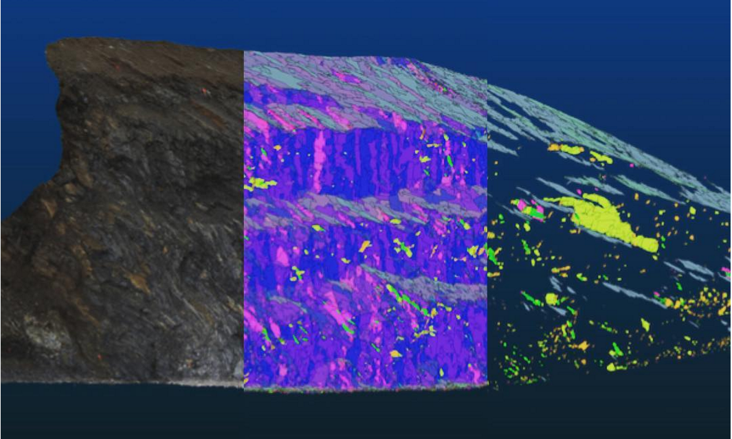
Amazing 3D images generated from a large number of 2D images of outcrop. LEft: the natural colour image. Middle: all facets generated by point cloud analysis. Right: the final set of human-filtered facets. © Joseph Cormier 2016

Amazing 3D images generated from a large number of 2D images of outcrop. LEft: the natural colour image. Middle: all facets generated by point cloud analysis. Right: the final set of human-filtered facets. © Joseph Cormier 2016

Probably the most eye-catching poster was that of Joseph Cormier (UNB), who is experimenting with computer-assisted structural interpretation. Using dozens of high-res photographs collected by a UAV, Joseph combines them to create reconstruct the 3D scene of the outcrop — just from photographs, no lidar or other ranging technology. The resulting point cloud reveals the orientations of the outcrop's faces, as well as fractures, exposed faults, and so on. A human interpreter can then apply her judgment to filter these facets to groups of tectonically significant sets, at which point they can be plotted on a stereonet. Beats crawling around with a Brunton or Suunto for days!

Hyperspectral imaging

There was another interesting poster by a local mining firm that I can't find in the abstract volume. They had some fine images from CoreScan, a hyperspectral imaging and analysis company operating in the mining industry. The technology, which can discern dozens of rock-forming minerals from their near infrared and shortwave infrared absorption characteristics, seems especially well-suited to mining, where mineralogical composition is usually more important than texture and sedimentological interpretation. 

Isabel Chavez (SMU) didn't need a commercial imaging service. To help correlate Laurasian shales on either side of the Atlantic, she presented results from using a handheld Konica-Minolta spectrophotometer on core. She found that CIE L* and a* colour parameters correlated with certain element ratios from ICP-MS analysis. Like many of the students at AGS, Isabel was presenting her undergraduate thesis — a real achievement.

Interesting aside: one of the chief applications of colour meters is measuring the colour of chips. Fascinating.

The hacker spirit is alive and well

The full spectrum (top), and the CCD responses with IR filter, Red filter, green filter, and blue filter (bottom). All of the filters admitted some infrared light, causing problems for calibration. © Robert McEwan 2016.

The full spectrum (top), and the CCD responses with IR filter, Red filter, green filter, and blue filter (bottom). All of the filters admitted some infrared light, causing problems for calibration. © Robert McEwan 2016.

After seeing those images, and wishing I had a hyperspectral imaging camera, Rob McEwan (Dalhousie) showed how to build one! In a wonderfully hackerish talk, he showed how he's building a $100 mineralogical analysis tool. He started by removing the IR filter from a second-hand Nikon D90, then — using a home-made grating spectrometer — measured the CCD's responses in the red, green, blue, and IR bands. After correcting the responses, Rob will use the USGS spectral library (Clark et al. 2007) to predict the contributions of various minerals to the image. He hopes to analyse field and lab photos at many scales. 

Once you have all this data, you also have to be able to process it. Joshua Wright (UNB) showed how he has built a suite of VisualBasic Macros to segment photomicrographs into regions representing grains using FIJI, then post-process the image data as giant arrays in an Excel spreadsheet (really!). I can see how a workflow like this might initially be more accessible to someone new to computer programming, but I felt like he may have passed Excel's sweetspot. The workflow would be much smoother in Python with scikit-image, or MATLAB with the Image Processing Toolbox. Maybe that's where he's heading. You can check out his impressive piece of work in a series of videos; here's the first:

Looking forward to 2016

All in all, the meeting was a good kick off to the geoscience year — a chance to catch up with some local geoscientists, and meet some new ones. I also had the chance to update the group on striplog, which generated a bit of interest. Now I'm back in Mahone Bay, enjoying the latest winter storm, enjoying the feeling of having something positive to blog about!

Please be aware that, unlike the images I usually include in posts, the images in this post are not open access and remain the copyright of their respective authors.


References

Isabel Chavez, David Piper, Georgia Pe-Piper, Yuanyuan Zhang, St Mary's University (2016). Black shale Selli Level recorded in Cretaceous Naskapi Member cores in the Scotian Basin. Oral presentation, AGS Colloquium, Truro NS, Canada.

Clark, R.N., Swayze, G.A., Wise, R., Livo, E., Hoefen, T., Kokaly, R., Sutley, S.J., 2007, USGS digital spectral library splib06a: U.S. Geological Survey, Digital Data Series 231

Joseph Cormier, Stefan Cruse, Tony Gilman, University of New Brunswick (2016). An optimized method of unmanned aerial vehicle surveying for rock slope analysis, 3D modeling, and structural feature extraction. Poster, AGS Colloquium, Truro NS, Canada.

Robert McEwan, Dalhousie University (2016). Detecting compositional variation in granites – a method for remotely sensed platform. Oral presentation, AGS Colloquium, Truro NS, Canada.

Joshua Wright, University of New Brunswick (2016). Using macros and advanced functions in Microsoft ExcelTM to work effectively and accurately with large data sets: An example using sulfide ore characterizatio. Oral presentation, AGS Colloquium, Truro NS, Canada.

Old skool plot tool

It's not very glamorous, but sometimes you just want to plot a SEG-Y file. That's why we crafted seisplot. OK, that's why we cobbled seisplot together out of various scripts and functions we had lying around, after a couple of years of blog posts and Leading Edge tutorials and the like.

Pupils of the old skool — when everyone knew how to write a bash script, pencil crayons and lead-filled beanbags ruled the desktop, and Carpal Tunnel Syndrome was just the opening act to the Beastie Boys — will enjoy seisplot. For a start, it's command line only: 

    python seisplot.py -R -c config.py ~/segy_files -o ~/plots

Isn't that... reassuring? In this age of iOS and Android and Oculus Rift... there's still the command line interface.

Features galore

So what sort of features can you look forward to? Other than all the usual things you've come to expect of subsurface software, like a complete lack of support or documentation. (LOL, I'm kidding.) Only these awesome selling points:

  • Make wiggle traces or variable density plots... or don't choose — do both!
  • If you want, the script will descend into subdirectories and make plots for every SEG-Y file it finds.
  • There are plenty of colourmaps to choose from, or if you're insane you can make your own.
  • You can make PNGs, JPGs, SVGs or PDFs. But not CGM, sorry about that.

Well, I say 'selling points', but the tool is 100% free. We think this is a fair price. It's also open source of course, so please — seriously, please — improve the source code, then share it with the world! The code is in GitHub, natch.

Never go full throwback

There is one more feature: you can go full throwback and add scribbles and coffee stains. Here's one for your wall:


The 2D seismic line in this post is from the USGS NPRA Seismic Data Archive, and are in the public domain. This is line number 31-81-PR (links directly to SEG-Y file).

White magic: calibrating seismic attributes

This post is part of a series on seismic attributes; the previous posts were...

  1. An attribute analysis primer
  2. Attribute analysis and statistics

Last time, I hinted that there might be a often-overlooked step in attribute analysis:

Calibration is a gaping void in many published workflows. How can we move past "that red blob looks like a point bar so I drew a line around it in PowerPoint" to "there's a 70% chance of finding reservoir quality sand at that location"?

Why is this step such a 'gaping void'? A few reasons:

  • It's fun playing with attributes, and you can make hundreds without a second thought. Some of them look pretty interesting, geological even. "That looks geological" is, however, not an attribute calibration technique. You have to prove it.
  • Nobody will be around when we find out the answer. There's a good chance that well will never be drilled, but when it is, you'll be on a different project, in a different company, or have left the industry altogether and be running a kayak rental business in Belize.
  • The bar is rather low. The fact that many published examples of attribute analysis include no proof at all, just a lot of maps with convincing-looking polygons on them, and claims of 'better reservoir quality over here'. 

This is getting discouraging. Let's look at an example. Now, it's hard to present this without seeming over-critical, but I know these gentlemen can handle it, and this was only a magazine article, so we needn't make too much of it. But it illustrates the sort of thing I'm talking about, so here goes.

Quoting from Chopra & Marfurt (AAPG Explorer, April 2014), edited slightly for brevity:

While coherence shows the edges of the channel, it gives little indication of the heterogeneity or uniformity of the channel fill. Notice the clear definition of this channel on the [texture attribute — homogeneity].
We interpret [the] low homogeneity feature [...] to be a point bar in the middle of the incised valley (green arrow). This internal architecture was not delineated by coherence.

A nice story, making two claims:

  1. The attribute incompletely represents the internal architecture of the channel.
  2. The labeled feature on the texture attribute is a point bar.

I know explorers have to be optimists, and geoscience is all about interpretation, but as scientists we must be skeptical optimists. Claims like this are nice hypotheses, but you have to take the cue: go off and prove them. Remember confirmation bias, and Feynman's words:

The first principle is that you must not fool yourself — and you are the easiest person to fool.

The twin powers

Making geological predictions with seismic attribute analysis requires two related workflows:

  1. Forward modeling — the best way to tune your intuition is to make a cartoonish model of the earth (2D, isotropic, homogeneous lithologies) and perform a simplified seismic experiment on it (convolutional, primaries only, noise-free). Then you can compare attribute behaviour to the known model.
  2. Calibration — you are looking for an explicit, quantitative relationship between a physical property you care about (porosity, lithology, fluid type, or whatever) and a seismic attribute. A common way to show this is with a cross-plot of the seismic amplitude against the physical property.

When these foundations are not there, we can be sure that one or more bad things will happen:

  • The relationship produces a lot of type I errors (false positives).
  • It produces a lot of type II error (false negatives).
  • It works at some wells and not at others.
  • You can't reproduce it with a forward model.
  • You can't explain it with physics.

As the industry shrivels and questions — as usual — the need for science and scientists, we have to become more stringent, more skeptical, and more rigorous. Doing anything else feeds the confirmation bias of the non-scientific continent. Because it says, loud and clear: geoscience is black magic.


The image is part of the figure from Chopra, S and K Marfurt (2014). Extracting information from texture attributes. AAPG Explorer, April 2014. It is copyright of the Authors and AAPG.

More highlights from SEG

On Monday I wrote that this year's Annual Meeting seemed subdued. And so it does... but as SEG continued this week, I started hearing some positive things. Vendors seemed pleasantly surprised that they had made some good contacts, perhaps as many as usual. The technical program was as packed as ever. And of course the many students here seemed to be enjoying themselves as much as ever. (New Orleans might be the coolest US city I've been to; it reminds me of Montreal. Sorry Austin.)

Quieter acquisition

Pramik et al. (of Geokinetics) reported on a new marine vibrator acquisition using their AquaVib source. This instrument has been around for a while, indeed it was first tested over 20 years ago by IVI and later Geco (e.g. see J Bird, TLE, June 2003). If perfected, it will allow for much quieter marine seismic acquisition, reducing harm to marine mammals, with no loss of quality (images below from their abstract and their copyright with SEG):

Ben told me one of his favourite talks was Schostak & Jenkerson with a report from a JIP (Shell, ExxonMobil, Total, and Texas A&M) trying to build a new marine vibrator.  Three designs are being tested by the current consortium, respectively manufactured by PGS with an electrical model, APS with a mechanical piston, and Teledyne with a bubble resonator.

In other news:

  • Talks at Dallas 2016 will only be 15 minutes long. Hopefully this is to allow room in the schedule for something else, not just more talks.
  • Dave Hale has retired from Colorado School of Mines, and apparently now 'writes software with Dean Witte'. So watch out for that!
  • A sure sign of industry austerity: "Would you like Bud Light, or Miller Light?"
  • Check out the awesome ribbons that some clever student thought of. I'm definitely pinching that idea.

That's all I have for now, and I'm flying home today so that's it for SEG 2015. I will be reporting on the hackathon soon I promise, and I'll try to get my paper on Pick This recorded next week (but here's a sneak peek). Stay tuned!


References

Bill Pramik, M. Lee Bell, Adam Grier, and Allen Lindsay (2015) Field testing the AquaVib: an alternate marine seismic source. SEG Technical Program Expanded Abstracts 2015: pp. 181-185. doi: 10.1190/segam2015-5925758.1

Brian Schostak* and Mike Jenkerson (2015) The Marine Vibrator Joint Industry Project. SEG Technical Program Expanded Abstracts 2015: pp. 4961-4962. doi: 10.1190/segam2015-6026289.1

The Rock Property Catalog again

Do you like data? Data about rocks? Open, accessible data that you can use for any purpose without asking? Read on.

After writing about anisotropy back in February, and then experimenting with storing rock properties in SubSurfWiki later that month, a few things happened:

  • The server I run the wiki on — legacy Amazon AWS infrastructure — crashed, and my backup strategy turned out to be <cough> flawed. It's now running on state-of-the-art Amazon servers. So my earlier efforts were mostly wiped out... Leaving the road clear for a new experiment!
  • I came across an amazing resource called Mudrock Anisotropy, or — more appealingly — Mr Anisotropy. Compiled by Steve Horne, it contains over 1000 records of rocks, gathered from the literature. It is also public domain and carries only a disclaimer. But it's a spreadsheet, and emailing a spreadsheet around is not sustainable.
  • The Common Ground database that was built by John A. Scales, Hans Ecke and Mike Batzle at Colorado School of Mines in the late 1990s, is now defunct and has been officially discontinued, as of about two weeks ago. It contains over 4000 records, and is public domain. The trouble is, you have to restore a SQLite database to use it.

All this was pointing towards a new experiment. I give you: the Rock Property Catalog again! This time it contains not 66 rocks, but 5095 rocks. Most of them have \(V_\mathrm{P}\), \(V_\mathrm{S}\) and  \(\rho\). Many of them have Thomsen's parameters too. Most have a lithology, and they all have a reference. Looking for Cretaceous shales in North America to use as analogs on your crossplots? There's a rock for that.

As before, you can query the catalog in various ways, either via the wiki or via the web API. Let's say we want to find shales with a velocity over 5000 m/s. You have a few options:

  1. Go to the semantic search form on the wiki and type [[lithology::shale]][[vp::>5000]]
  2. Make a so-called inline query on your own wiki page (you need an account for this).
  3. Make a query via the web API with a rather long URL: http://www.subsurfwiki.org/api.php?action=ask&query=[[RPC:%2B]][[lithology::shale]][[Vp::>5000]]|%3FVp|%3FVs|%3FRho&format=jsonfm

I updated the Jupyter Notebook I published last time with a new query. It's pretty hacky. I'll work on this to produce a more robust method, with some error handling and cleaner code — stay tuned.

The database supports lots of properties, including:

  • Citation and reference
  • Description, lithology, colour (you can have pictures if you want!)
  • Location, lat/lon, basin, age, depth
  • Vp, Vs, \(\rho\), as well as \(\rho_\mathrm{dry}\) and \(\rho_\mathrm{grain}\)
  • Thomsen's \(\epsilon\), \(\delta\), and \(\gamma\)
  • Static and dynamic Young's modulus and Poisson ratio
  • Confining pressure, pore pressure, effective stress, axial stress
  • Frequency
  • Fluid, saturation type, saturation
  • Porosity, permeability, temperature
  • Composition

There is more from the Common Ground data to add, especially photographs. But for now, I'd love some feedback: is this the right set of properties? Do we need more? I want this to be useful — what kind of data and metadata would you like to see? 

I'll end with the usual appeal — I'm open to any kind of suggestions or help with this. Perhaps you can contribute new rocks, or a paper containing data? Or maybe you have some wiki skills, or can help write bots to improve the data? What can you bring? 

What is AVO-friendly processing?

It's the Geophysics Hackathon next month! Come down to Propeller in New Orleans on 17 and 18 October, and we'll feed you and give you space to build something cool. You might even win a prize. Sign up — it's free!

Thank you to the sponsors, OpenGeoSolutions and Palladium Consulting — both fantastic outfits. Hire them.

AVO-friendly processing gets called various things: true amplitude, amplitude-friendly, and controlled amplitude, controlled phase (or just 'CACP'). And, if you've been involved in any processing jobs you'll notice these phrases get thrown around a lot. But seismic geophysics has a dirty little secret... we don't know exactly what it is. Or, at least, we can't agree on it.

A LinkedIn discussion in the Seismic Data Processing group earlier this month prompted this post:

I can't compile a list of exactly which processes will harm your AVO analysis (can anyone? Has anyone??), but I think I can start a list of things that you need to approach with caution and skepticism:

  • Anything that is not surface consistent. What does that mean? According to Oliver Kuhn (now at Quantec in Toronto):
Surface consistent: a shot-related [process] affects all traces within a shot gather in the same way, independent of their receiver positions, and, a receiver-related [process] affects all traces within a receiver gather in the same way, independent of their shot positions.
  • Anything with a window — spatial or temporal. If you must use windows, make them larger or longer than your areas and zones of interest. In this way, relative effects should be preserved.
  • Anything that puts the flattening of gathers before the accuracy of the data (<cough> trim statics). Some flat gathers don't look flat. (The thumbnail image for this post is from Duncan Emsley's essay in 52 Things.)
  • Anything that is a sort of last resort, post hoc attempt to improve the data — what we might call 'cosmetic' treatments. Things like wavelet stretch correction and spectral shaping are good for structural interpreters, but not for seismic analysts. At the very least, get volumes without them, and convince yourself they did no harm.
  • Anything of which people say, "This should be fine!" but offer no evidence.

Back to my fourth point there... spectral shaping and wavelet stretch correction (e.g. this patented technique I was introduced to at ConocoPhillips) have been the subject of quite a bit of discussion, in my experience. I don't know why; both are fairly easy to model, on the face of it. The problem is that we start to get into the sticky question of what wavelets 'see' and what's a wavelet anyway, and hang on a minute why does seismic reflection even work? Personally, I'm skeptical, especially as we get more used to, and better at, looking at spectral decompositions of stacked and pre-stack data.

Divergent paths

I have seen people use seismic data with very different processing paths for structural interpretation and for AVO analysis. This can happen on long-term projects, where the structural framework depends on an old post-stack migration that was later reprocessed for AVO friendliness. This is a bad idea — you won't be able to put the quantitative results into the structural framework without introducing substantial error.

What we need is a clinical trial of processing algorithms, in which they are tested against a known model like Marmousi, and their effect on attributes is documented. If such studies exist, I'd love to hear about them. Come to think of it, this would make a good topic for a hackathon some day... Maybe Dallas 2016?

The hack is back: learn new skills in New Orleans

Looking for a way to broaden your skills for the next phase of your career? Need some networking that isn't just exchanging business cards? Maybe you just need a reminder that subsurface geoscience is the funnest thing ever? I have something for you...

It's the third Geophysics Hackathon! The most creative geoscience event of the year. Completely free, as always, and fun for everyone — not just programmers. So mark your calendar for the weekend of 17 and 18 October, sign up on your own or with a team, and come to New Orleans for the most creative 48 hours of your career so far.

What is a hackathon?

It's a fun, 2-day event full of geophysics and tech. Most people participate in teams of up to 4 people, but you can take part on your own too. There's plenty of time on the first morning to find projects to work on, or maybe you already have something in mind. At the end of the second day, we show each other what we've been working on with a short demo. There are some fun prizes for especially interesting projects.

You don't have to be a programmer to join the fun. If you're more into geological interpretation, or reservoir engineering, or graphic design, or coming up with amazing ideas — there's a place for you at the hackathon. 

FAQ

  • How much does it cost? It's completely free!
  • I don't believe you. Believe it. Coffee and tacos will be provided. Just bring a laptop.
  • When is it? 17 and 18 October, doors open at 8 am each day, and we go till about 5.30.
  • So I won't miss the SEG Icebreaker? No, we'll all go!
  • Where is it? Propeller, 4035 Washington Avenue, New Orleans
  • How do I sign up? Find out more and register for the event at ageo.co/geohack15

Being part of it all

If this all sounds awesome to you, and you'll be in New Orleans this October, sign up! If you don't think it's for you, please drop in for a visit and a coffee — give me a chance to convince you to sign up next time.

If you own or work for an organization that wants to see more innovation in the world, please think about sponsoring this event, or a future one.

Last thing: I'd really appreciate any signal boost you can offer — please consider forwarding this post to the most creative geoscientist you know, especially if they're in the Houston and New Orleans area. I'm hoping that, with your help, this can be our biggest event ever.

How to QC a seismic volume

I've had two emails recently about quality checking seismic volumes. And last month, this question popped up on LinkedIn:

We have written before about making a data quality volume for your seismic — a handy way to incorporate uncertainty into risk maps — but these recent questions seem more concerned with checking a new volume for problems.

First things first

Ideally, you'd get to check the volume before delivery (at the processing shop, say), otherwise you might have to actually get it loaded before you can perform your QC. I am assuming you've already been through the processing, so you've seen shot gathers, common-offset gathers, etc. This is all about the stack. Nonetheless, the processor needs to prepare some things:

  • The stack volume, of course, with and without any 'cosmetic' filters (eg fxy, fk).
  • A semblance (coherency, similarity, whatever) volume.
  • A fold volume.
  • Make sure the processor has some software that can rapidly scan the data, plot amplitude histograms, compute a spectrum, pick a horizon, and compute phase. If not, install OpendTect (everyone should have it anyway), or you'll have to load the volume yourself.

There are also some things you can do ahead of time. 

  1. Be part of the processing from the start. You don't want big surprises at this stage. If a few lines got garbled during file creation, no problem. If there's a problem with ground-roll attentuation, you're not going to be very popular.
  2. Make sure you know how the survey was designed — where the corners are, where you would expect live traces to be, and which way the shot and receiver lines went (if it was an orthogonal design). Get maps, take them with you.
  3. Double-check the survey parameters. The initial design was probably changed. The PowerPoint presentation was never updated. The processor probably has the wrong information. General rule with subsurface data: all metadata is probably wrong. Ideally, talk to someone who was involved in the planning of the survey.
  4. You didn't skip (2) did you? I'm serious, double check everything.

Crack open the data

OK, now you are ready for a visit with the processor. Don't fall into the trap of looking at the geology though — it will seduce you (it's always pretty, especially if it's the first time you've seen it). There is work to do first.

  1. Check the cornerpoints of the survey. I like the (0, 0) trace at the SW corner. The inline and crossline numbering should be intuitive and simple. Make sure the survey is the correct way around with respect to north.
  2. Scan through timeslices. All of them. Is the sample interval what you were expecting? Do you reach the maximum time you expected, based on the design? Make sure the traces you expect to be live are live, and the ones you expect to be dead are dead. Check for acquisition footprint. Start with greyscale, then try another colourmap.
  3. Repeat (5) but in a similarity volume (or semblance, coherency, whatever). Look for edges, and geometric shapes. Check again for footprint.
  4. Look through the inlines and crosslines. These usually look OK, because it's what processors tend to focus on.
  5. Repeat (7) but in a similarity volume.

Dive into the details

  1. Check some spectrums. Select some subsets of the data — at least 100 traces and 1000 ms from shallow, deep, north, south, east, west — and check the average spectrums. There should be no conspicuous notches or spikes, which could be signs of all sorts of things from poorly applied filters to reverberation.
  2. Check the amplitude histograms from those same subsets. It should be 32-bit data — accept no less. Check the scaling — the numbers don't mean anything, so you can make them range over whatever you like. Something like ±100 or ±1000 tends to make for convenient scaling of amplitude maps and so on; ±1.0 or less can be fiddly in some software. Check for any departures from an approximately Laplacian (double exponential) distribution: clipping, regular or irregular spikes, or a skewed or off-centre distribution:
  1. Interpret a horizon and check its phase. See Purves (Leading Edge, October 2014) or SubSurfWiki for some advice.
  2. By this time, the fold volume should yield no surprises. If any of the rest of this checklist throws up problems, the fold volume might help troubleshoot.
  3. Check any other products you asked for. If you asked for gathers or angle stacks (you should), check them too.

Last of all, before actual delivery, talk to whoever will be loading the data about what kind of media they prefer, and what kind of file organization. They may also have some preferences for the contents of the SEG-Y file and trace headers. Pass all of this on to the processor. And don't forget to ask for All The Seismic

What about you?

Have I forgotten anything? Are there things you always do to check a new seismic volume? Or if you're really brave, maybe you have some pitfalls or even horror stories to share...

Introducing Bruges

bruges_rooves.png

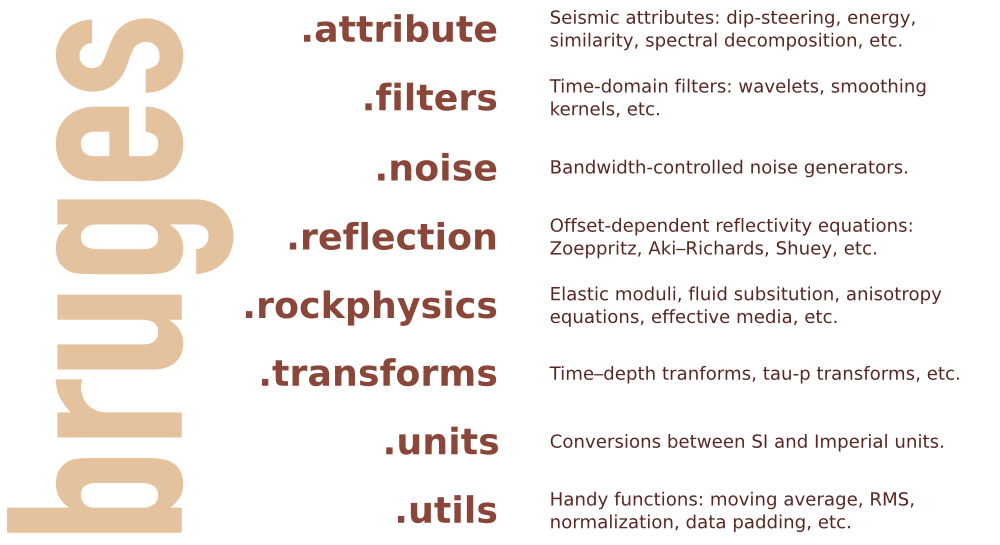
Welcome to Bruges, a Python library (previously known as agilegeo) that contains a variety of geophysical equations used in processing, modeling and analysing seismic reflection and well log data. Here's what's in the box so far, with new stuff being added every week:


Simple AVO example

VP [m/s] VS [m/s] ρ [kg/m3]
Rock 1 3300 1500 2400
Rock 2 3050 1400 2075

Imagine we're studying the interface between the two layers whose rock properties are shown here...

To compute the zero-offset reflection coefficient at zero offset, we pass our rock properties into the Aki-Richards equation and set the incident angle to zero:

 >>> import bruges as b
 >>> b.reflection.akirichards(vp1, vs1, rho1, vp2, vs2, rho2, theta1=0)
 -0.111995777064

Similarly, compute the reflection coefficient at 30 degrees:

 >>> b.reflection.akirichards(vp1, vs1, rho1, vp2, vs2, rho2, theta1=30)
 -0.0965206980095

To calculate the reflection coefficients for a series of angles, we can pass in a list:

 >>> b.reflection.akirichards(vp1, vs1, rho1, vp2, vs2, rho2, theta1=[0,10,20,30])
 [-0.11199578 -0.10982911 -0.10398651 -0.0965207 ]

Similarly, we could compute all the reflection coefficients for all incidence angles from 0 to 70 degrees, in one degree increments, by passing in a range:

 >>> b.reflection.akirichards(vp1, vs1, rho1, vp2, vs2, rho2, theta1=range(70))
 [-0.11199578 -0.11197358 -0.11190703 ... -0.16646998 -0.17619878 -0.18696428]

A few more lines of code, shown in the Jupyter notebook, and we can make some plots:


Elastic moduli calculations

With the same set of rocks in the table above we could quickly calculate the Lamé parameters λ and µ, say for the first rock, like so (in SI units),

 >>> b.rockphysics.lam(vp1, vs1, rho1), b.rockphysics.mu(vp1, vs1, rho1)
 15336000000.0 5400000000.0

Sure, the equations for λ and µ in terms of P-wave velocity, S-wave velocity, and density are pretty straightforward: 


but there are many other elastic moduli formulations that aren't. Bruges knows all of them, even the weird ones in terms of E and λ.


All of these examples, and lots of others — Backus averaging,  examples are available in this Jupyter notebook, if you'd like to work through them on your own.


Bruges is a...

It is very much early days for Bruges, but the goal is to expose all the geophysical equations that geophysicists like us depend on in their daily work. If you can't find what you're looking for, tell us what's missing, and together, we'll make it grow.

What's a handy geophysical equation that you employ in your work? Let us know in the comments!

Seismic inception

A month ago, some engineers at Google blogged about how they had turned a deep learning network in on itself and produced some fascinating and/or disturbing images:

One of the images produced by the team at Google. Click to see a larger version. Read more. CC-BY.

The basic recipe, which Google later open sourced, involves training a deep learning network (basically a multi-layer neural network) on some labeled images, animals maybe, then searching for matching patterns in a target image, like these clouds. If it finds something, it emphasizes it — given the data, it tries to construct an animal. Then do it again.

Or, here's how a Google programmer puts it (one of my favourite sentences ever)...

Making the "dream" images is very simple. Essentially it is just a gradient ascent process that tries to maximize the L2 norm of activations of a particular DNN layer. 

That's all! Anyway, the point is that you get utter weirdness:

OK, cool... what happens if you feed it seismic?

That was my first thought, I'm sure it was yours too. The second thing I thought, and the third, and the fourth, was: wow, this software is hard to compile. I spent an unreasonable amount of time getting caffe, the Berkeley Vision & Learning Centre's deep learning software, working. But on Friday I cracked it, so today I got to satisfy my curiosity.

The short answer is: reptiles. These weirdos were 8 levels down, which takes about 20 minutes to reach on my iMac.

Seismic data from the Virtual Seismic Atlas, courtesy of Fugro. 

THE DEEPDREAM TREATMENT. Mostly reptiles.

Er, right... what's the point in all this?

That's a good question. It's just a bit of fun really. But it makes you wonder:

  • What if we train the network on seismic facies? I think this could be very interesting.
  • Better yet, what if we train it on geology? Probably spurious: seismic is not geology.
  • Does this mean learning networks are just dumb machines, or can they see more than us? Tough one — human vision is highly fallible. There are endless illusions to prove this. But computers only do what we tell them, at least for now. I think if we're careful what we ask for, we can use these highly non-linear data-crunching algorithms for good.
  • Are we out of a job? Definitely not. How do you think machines will know what to learn? The challenge here is to make this work, and then figure out how it can help change, or at least accelerate, our understanding of the subsurface.

This deep learning stuff — of which the University of Toronto was a major pioneer during its emergence in about 2010 — is part of the machine learning revolution that you are, like it or not, experiencing. It will take time, and it will make awful mistakes, but the indications are that machine learning will eat every analytical method for breakfast. Customer behaviour prediction, computer vision, natural language processing, all this stuff is reeling from the relatively sudden and widespread availability of inexpensive computer intelligence. 

So what are we going to do with that?

&nbsp; &nbsp; &nbsp; &nbsp; &nbsp; &nbsp;Okay, one more. from Paige Bailey's Twitter feed.

           Okay, one more. from Paige Bailey's Twitter feed.