On being the world's smallest technical publishing company

Four months ago we launched our first book, 52 Things You Should Know About Geophysics. This little book contains 52 short essays by 37 amazing geoscientists. And me and Evan. 

Since it launched, we've been having fun hearing from people who have enjoyed it:

Yesterday's mail brought me an envelope from Stavanger — Matteo Niccoli sent me a copy of 52 Things. In doing so he beat me to the punch as I've been meaning to purchase a copy for some time. It's a good thing I didn't buy one — I'd like to buy a dozen. [a Calgary geoscientist]

A really valuable collection of advice from the elite in Geophysics to help you on your way to becoming a better more competent Geophysicist. [a review on Amazon.co.uk]

We are interested in ordering 50 to 100 copies of the book 52 Things You Should Know About Geophysics [from an E&P company. They later ordered 100.]

The economics

We thought some people might be interested in the economics of self-publishing. If you want to know more, please ask in the comments — we're happy to share our experiences. 

We didn't approach a publisher with our book. We knew we wanted to bootstrap and learn — the Agile way. Before going with Amazon's CreateSpace platform, we considered Lightning Source (another print-on-demand provider), and an ordinary 'web press' printer in China. The advantages of CreateSpace are Amazon's obvious global reach, and not having to carry any inventory. The advantages of a web press are the low printing cost per book and the range of options — recycled paper, matte finish, gatefold cover, and so on.

So, what does a book cost?

• You could publish a book this way for $0. But, unless you're an editor and designer, you might be a bit disappointed with your results. We spent about $4000 making the book: interior design about $2000, cover design was about $650, indexing about $450. We lease the publishing software (Adobe InDesign) for about $35 per month.
• Each book costs $2.43 to manufacture. Books are printed just in time — Amazon's machines must be truly amazing. I'd love to see them in action. 
• The cover price is $19 at Amazon.com, about €15 at Amazon's European stores, and £12 at Amazon.co.uk. Amazon are free to offer whatever discounts they like, at their expense (currently 10% at Amazon.com). And of course you can get free shipping. Amazon charges a 40% fee, so after we pay for the manufacturing, we're left with about $8 per book. 
• We also sell through our own estore, at $19. This is just a slightly customizable Amazon page. This channel is good for us because Amazon only charges 20% of the sale price as their fee. So we make about $12 per book this way. We can give discounts here too — for large orders, and for the authors.
• Amazon also sells the book through a so-called expanded distribution channel, which puts the book on other websites and even into bookstores (highly unlikely in our case). Unfortunately, it doesn't give us access to universities and libraries. Amazon's take is 60% through this channel.
• We sell a Kindle edition for $9. This is a bargain, by the way—making an attractive and functional ebook was not easy. The images and equations look terrible, ebook typography is poor, and it just feels less like a book, so we felt $9 was about right. The physical book is much nicer. Kindle royalties are complicated, but we make about $5 per sale. 

By the numbers

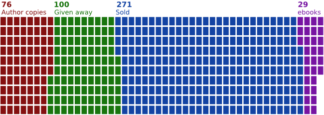
It doesn't pay to fixate on metrics—most of the things we care about are impossible to measure. But we're quantitative people, and numbers are hard to resist. To recoup our costs, not counting the time we lovingly invested, we need to sell 632 books. (Coincidentally, this is about how many people visit agilegeoscience.com every week.) As of right now, there are 476 books out there 'in the wild', 271 of which were sold for actual money. That's a good audience of people — picture them, sitting there, reading about geophysics, just for the love of it.

The bottom line

My wife Kara is an experienced non-fiction publisher. She's worked all over the world in editorial and production. So we knew what we were getting into, more or less. The print-on-demand stuff was new to her, and the retail side of things. We already knew we suck at marketing. But the point is, we knew we weren't in this for the money, and it's about relevant and interesting books, not marketing.

And now we know what we're doing. Sorta. We're in the process of collecting 52 Things about geology, and are planning others. So we're in this for one or two more whatever happens, and we hope we get to do many more.

We can't say this often enough: Thank You to our wonderful authors. And Thank You to everyone who has put down some hard-earned cash for a copy. You are awesome. 

Cross plots: a non-answer

On Monday I asked whether we should make crossplots according to statistical rules or natural rules. There was some fun discussion, and some awesome computation from Henry Herrera, and a couple of gems:

Physics likes math, but math doesn't care about physics — @jeffersonite

But... when I consider the intercept point I cannot possibly imagine a rock that has high porosity and zero impedance — Matteo Niccoli, aka @My_Carta

I tried asking on Stack Overflow once, but didn’t really get to the bottom of it, or perhaps I just wasn't convinced. The consensus seems to be that the statistical answer is to put porosity on y-axis, because that way you minimize the prediction error on porosity. But I feel—and this is just my flaky intuition talking—like this fails to represent nature (whatever that means) and so maybe that error reduction is spurious somehow.

Reversing the plot to what I think of as the natural, causation-respecting plot may not be that unreasonable. It's effectively the same as reducing the error on what was x (that is, impedance), instead of y. Since impedance is our measured data, we could say this regression respects the measured data more than the statistical, non-causation-respecting plot.

So must we choose? Minimize the error on the prediction, or minimize the error on the predictor. Let's see. In the plot on the right, I used the two methods to predict porosity at the red points from the blue. That is, I did the regression on the blue points; the red points are my blind data (new wells, perhaps). Surprisingly, the statistical method gives an RMS error of 0.034, the natural method 0.023. So my intuition is vindicated! 

Unfortunately if I reverse the datasets and instead model the red points, then predict the blue, the effect is also reversed: the statistical method does better with 0.029 instead of 0.034. So my intuition is wounded once more, and limps off for an early bath.

Irreducible error?

Here's what I think: there's an irreducible error of prediction. We can beg, borrow or steal error from one variable, but then it goes on the other. It's reminiscent of Heisenberg's uncertainty principle, but in this case, we can't have arbitrarily precise forecasts from imperfectly correlated data. So what can we do? Pick a method, justify it to yourself, test your assumptions, and then be consistent. And report your errors at every step. 

I'm reminded of the adage 'Correlation does not equal causation.' Indeed. And, to borrow @jeffersonite's phrase, it seems correlation also does not care about causation.

Cross plot or plot cross?

I am stumped. About once a year, for the last nine years or so, I have failed to figure this out.

What could be simpler than predicting porosity from acoustic impedance? Well, lots of things, but let’s pretend for a minute that it’s easy. Here’s what you do:

1.   Measure impedance at a bunch of wells
2.   Measure the porosity — at seismic scale of course — at those wells
3.   Make a crossplot with porosity on the y-axis and amplitude on the x-axis
4.   Plot the data points and plot the regression line (let’s keep it linear)
5.   Find the equation of the line, which is of the form y = ax + b, or porosity = gradient × impedance + constant
6.   Apply the equation to a map (or volume, if you like) of amplitude, and Bob's your uncle.

Easy!

But, wait a minute. Is Bob your uncle after all? The parameter on the y-axis is also called the dependent variable, and that on the x-axis the independent. In other words, the crossplot represents a relationship of dependency, or causation. Well, porosity certainly does not depend on impedance — it’s the other way around. To put it another way, impedance is not the cause of porosity. So the natural relationship should put impedance, not porosity, on the y-axis. Right?

Therefore we should change some steps:

3.   Make a crossplot with impedance on the y-axis and porosity on the x-axis
4.   Plot the data points and plot the regression line
5a. Find the equation of the line, which is of the form y = ax + b, or impedance = gradient × porosity + constant
5b. Rearrange the equation for what we really want:
porosity = (impedance – constant)/gradient

Not quite as easy! But still easy.

More importantly, this gives a different answer. Bob is not your uncle after all. Bob is your aunt. To be clear: you will compute different porosities with these two approaches. So then we have to ask: which is correct? Or rather, since neither going to give us the ‘correct’ porosity, which is better? Which is more physical? Do we care about physicality?

I genuinely do not know the answer to this question. Do you?

If you're interested in playing with this problem, the data I used are from Imaging reservoir quality seismic signatures of geologic effects, report number DE-FC26-04NT15506 for the US Department of Energy by Gary Mavko et al. at Stanford University. I digitized their figure D-8; you can download the data as a CSV here. I have only plotted half of the data points, so I can use the rest as a blind test. 

Update on 2012-09-20 00:23 by Matt Hall

Don't miss my follow up to this post... a non-answer. More input and discussion always welcome! 

The intentional professional

I'm involved in a local effort to launch a coworking and business incubation space in Mahone Bay, Nova Scotia, where I live. Like most things worth doing, it's taking some time, but I think we'll get there eventually. Along this journey, I heard a lovely phrase recently — intentional community. What a great way to describe a group of coworkers and entrepreneurs, implying a group formed not just on purpose, but also with purpose. 

But it made me think too — it made me wonder if some of the communities I'm involved in might be unintentional — accidental, inadvertent, perhaps even a mistake? Would you describe your workplace as intentional? If you're a student, are your classes intentional? That committee you're on — is that intentional?

Another phrase that keeps popping into my head lately is

Don't be a looky-loo. — Clay Shirky, Cognitive Surplus

Even if you don't know what a looky-loo is, you'll recognize the behaviour immediately. A looky-loo is someone who, taking Woody Allen's advice a little too seriously, thinks 80% of success is showing up. If you've ever organized a meeting, with an idea that you might get something done in it, you know the sort: they arrive, they eat the cookies, they do the small talk, then they sit there and stare at you for an hour, then they leave. No input given. No notes taken. No point being there. 

Next time you hear yourself described in passive terms — attendee, reader, employee, student, user, consumer, react to it. You're being described as a person that things happen to. A victim.

Instead of being an unintentional victim, think of yourself an essential part of whatever it is. You are a participant, a partner, a stakeholder, a contributor, a collaborator. If you're not an essential part of it then, for everyone's sake, don't go.

This is what professionalism is. 

Great geophysicists #5: Huygens

Christiaan Huygens was a Dutch physicist. He was born in The Hague on 14 April 1629, and died there on 8 July 1695. It's fun to imagine these times: he was a little older than Newton (born 1643), a little younger than Fermat (1601), and about the same age as Hooke (1635). He lived in England and France and must have met these men.

It's also fun to imagine the intellectual wonder life must have held for a wealthy, educated person in these protolithic Enlightenment years. Everyone, it seems, was a polymath: Huygens made substantial contributions to probability, mechanics, astronomy, optics, and horology. He was the first to describe Saturn's rings. He invented the pendulum clock. 

Then again, he also tried to build a combustion engine that ran on gunpowder. 

Geophysicists (and most other physicists) know him for his work on wave theory, which prevailed over Newton's corpuscles—at least until quantum theory. In his Treatise on Light, Huygens described a model for light waves that predicted the effects of reflection and refraction. Interference has to wait 38 years till Fresnel. He even explained birefringence, the anisotropy that gives rise to the double-refraction in calcite.

The model that we call the Huygens–Fresnel principle consists of spherical waves emanating from every point in a light source, such as a candle's flame. The sum of these manifold wavefronts predicts the distribution of the wave everywhere and at all times in the future. It's a sort of infinitesimal calculus for waves. I bet Newton secretly wished he'd thought of it.

Fold for sale

A few weeks ago I wrote a bit about seismic fold, and why it's important for seeing through noise. But how do you figure out the fold of a seismic survey?

The first thing you need to read is Norm Cooper's terrific two-part land seismic tutorial. One of his main points is that it's not really fold we should worry about, it's trace density. Essentially, this normalizes the fold by the area of the natural bins (the areal patches into which we will gather traces for the stack). Computing trace density, given effective maximum offset X_max (or depth, in a pinch), source and receiver line spacings S and R, and source and receiver station intervals s and r:

Cooper helpfully gave ballpark ranges for increasingly hard imaging problems. I've augmented it, based on my own experience. Your mileage may vary! (Edit this table)

Traces cost money

So we want more traces. The trouble is, traces cost money. The chart below reflects my experiences in the bitumen sands of northern Alberta (as related in Hall 2007). The model I'm using is a square land 3D with an orthogonal geometry and no overlaps (that is, a single swath), and 2007 prices. A trace density of 50 traces/km² is equivalent to a fold of 5 at 500 m depth. As you see, the cost of seismic increases as we buy more traces for the stack. Fun fact: at a density of about 160 000 traces/km², the cost is exactly $1 per trace. The good news is that it increases with the square root (more or less), so the incremental cost of adding more traces gets progressively cheaper:

Given that you have limited resources, your best strategy for hitting the 'sweet spot'—if there is one—is lots and lots of testing. Keep careful track of what things cost, so you can compute the probable cost benefit of, say, halving the trace density. With good processing, you'll be amazed what you can get away with, but of course you risk coping badly with unexpected problems in the near surface.

What do you think? How do you make decisions about seismic geometry and trace density?

References

Cooper, N (2004). A world of reality—Designing land 3D programs for signal, noise, and prestack migration, Parts 1 and 2. The Leading Edge. October and December, 2004. 

Hall, M (2007). Cost-effective, fit-for-purpose, lease-wide 3D seismic at Surmont. SEG Development and Production Forum, Edmonton, Canada, July 2007.

Geothermal facies from seismic

Here is a condensed video of the talk I gave at the SEG IQ Earth Forum in Colorado. Much like the tea-towel mock-ups I blogged about in July, this method illuminates physical features in seismic by exposing hidden signals and textures. 

This approach is useful for photographs of rocks and core, for satellite photography, or any geophysical data set, when there is more information to be had than rectangular and isolated arrangements of pixel values.

Click to download slides with notes!Interpretation has become an empty word in geoscience. Like so many other buzzwords, instead of being descriptive and specific jargon, it seems that everyone has their own definition or (mis)use of the word. If interpretation is the art and process of making mindful leaps between unknowns in data, I say, let's quantify to the best of our ability the data we have. Your interpretation should be iteratable, it should be systematic, and it should be cast as an algorithm. It should be verifiable, it should be reproducible. In a word, scientific.  

You can download a copy of the presentation with speaking notes, and access the clustering and texture codes on GitHub. 

News of the month

Like the full moon, our semi-regular news round-up has its second outing this month. News tips?

New software releases

QGIS, our favourite open source desktop GIS too, moves to v1.8 Lisboa. It gains pattern fills, terrain analysis, layer grouping, and lots of other things.

Midland Valley, according to their June newsletter, will put Move 2013 on the Mac, and they're working on iOS and Android versions too. Multi-platform keeps you agile. 

New online tools

The British Geological Survey launched their new borehole viewer for accessing data from the UK's hundreds of shallow holes. Available on mobile platforms too, this is how you do open data, staying relevant and useful to people.

Joanneum Research, whose talk at EAGE I mentioned, is launching their seismic attributes database seismic-attribute.info as a €6000/year consortium, according to an email we got this morning. Agile* won't be joining, we're too in love with Mendeley's platform, but maybe you'd like to — enquire by email.

Moar geoscience jobs

Neftex, a big geoscience consulting and research shop based in Oxford, UK, is growing. Already with over 80 people, they expect to hire another 50 or so. That's a lot of geologists and geophysicists! And Oxford is a lovely part of the world.

Ikon is opening a Canada office in Calgary. Ikon Science Canada Ltd is born! Contact Rob Dudley on rdudley@ikonscience.com for more info.

— Ikon Science America (@IkonAmericas) August 24, 2012

Ikon Science, another UK subsurface consulting and research firm, is opening a Calgary office. We're encouraged to see that they chose to announce this news on Twitter — progressive!

This regular news feature is for information only. We aren't connected with any of these organizations, and don't necessarily endorse their products or services. Except QGIS, which we definitely do endorse, cuz it's awesome. 

Cut the small print

We received a contract for a new piece of work recently. This wouldn't normally be worth remarking on, but this contract was special. It was different. It was 52 pages long.

It was so comically long that the contracts analyst at the company that sent it to me actually called me up before sending it to say, "The contract is comically long. It's just standard procedure. Sorry." Because it's so long, it's effectively all small print — if there's anything important in there, I'm unlikely to see it. The document bullies me into submission. I give in.

Unfortunately, this is a familiar story. Some (mostly non-lawyers) like Alan Siegel are trying to change it:

Before we all laugh derisively at lawyers, wait a second. Are you sure that everyone reads every word in your reports and emails? Do they look at every slide in your presentations? Do they listen to every word in your talks? 

If you suspect they don't, ask yourself why not. And then cut. Cut until all that's left is what matters. If there's other important stuff — exceptions, examples, footnotes, small print, legal jargon — move it somewhere and give people a link.

Shales and technology

Day three of the SEG IQ Earth Forum had more organizational diversity than the previous two days. The morning session was on seismic for unconventional plays. This afternoon was for showcasing novel implementations of seismic attributes.

Resource shale plays aren’t as wildly economic as people think. This is not only because geology is complex and heterogeneous, but also because drilling and completions processes aren't constant either. Robin Pearson from Anadarko presented a wonderful shale gas science experiment: three systematic field tests designed to target key uncertainties:

• List all of your uncertainties and come up with a single test for evaluating each, holding all other variables constant.
• Make sure you collect enough data so that results are statistically valid.
• Make your experiment scalable — 10 measurements must be extrapolatable to influence hundreds.

To better understand production heterogeniety, they drilled and fracked three wells in exactly the same way. Logging and microseismic surface monitoring showed a tight limestone zone that was liberating gas from a strike slip fault, previously unseen. 

The best talk for interpreters so far was from Randy Pepper, who has done basin-scale modeling to define the erosional and non-depositional periods of geologic history not captured in the rock record. He used Wheeler diagrams to transform between two different representations of the same data, so that interpreters could work interactively between the structural and stratigraphic domains. It reminded me of dGB's Horizon Cube technology, allowing interpreters to explore between the mappable horizons in their data. Next step: allowing interpreters to perturb structural restorations on the fly. 

If you showed a seismic amplitude map to a radiologist, they might form completely rational arguments for arteries and other anatomical structures. Interpreters sometimes see what they want to see, which can be a problem. My favorite talk so far was from Jonathan Henderson from ffa. He is dedicated to keeping art and expertise in the interpretation process. His company has developed software for building data-guided geobodies with an organic and intuitive design. Automatic data classification can only go so far in elucidating what the human brain can perceive. Read his article.

I repeat his principles here:

• Understanding the imaged geology: the art of interpretation,
• Measurements and Uncertainty: a need for science
• Adaptive Geobodies: combining art and science.

Kudos to John for ending the talk with a video demo of the software in action. Gasps from the crowd were a plenty. I'm hoping for more of this tomorrow!