What is SEG-Y?

The confusion starts with the name, but whether you write SEGY, SEG Y, or SEG-Y, it's probably definitely pronounced 'segg why'. So what is this strange substance?

SEG-Y means seismic data. For many of us, it's the only type of seismic file we have much to do with — we might handle others, but for the most part they are closed, proprietary formats that 'just work' in the application they belong to (Landmark's brick files, say, or OpendTect's CBVS files). Processors care about other kinds of data — the SEG has defined formats for field data (SEG-D) and positional data (SEG-P), for example. But SEG-Y is the seismic file for everyone. Kind of.

The open SEG-Y "standard" (those air quotes are an important feature of the standard) was defined by SEG in 1975. The first revision, Rev 1, was published in 2002. The second revision, Rev 2, was announced by the SEG Technical Standards Committee at the SEG Annual Meeting in 2013 and I imagine we'll start to see people using it in 2014. 

What's in a SEG-Y file?

SEG-Y files have lots of parts:

The important bits are the EBCDIC header (green) and the traces (light and dark blue).

The EBCDIC text header is a rich source of accurate information that provides everything you need to load your data without problems. Yay standards!

Oh, wait. The EBCDIC header doesn't say what the coordinate system is. Oh, and the datum is different from the processing report. And the dates look wrong, and the trace length is definitely wrong, and... aargh, standards!

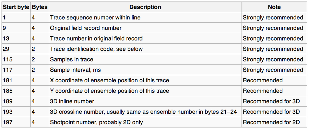
The other important bit — the point of the whole file really — is the traces themselves. They also have two parts: a header (light blue, above) and the actual data (darker blue). The data are stored on the file in (usually) 4-byte 'words'. Each word has its own address, or 'byte location' (a number), and a meaning. The headers map the meaning to the location, e.g. the crossline number is stored in byte 21. Usually. Well, sometimes. OK, it was one time.

According to the standard, here's where the important stuff is supposed to be:

I won't go into the unpleasantness of poking around in SEG-Y files right now — I'll save that for next time. Suffice to say that it's often messy, and if you have access to a data-loading guru, treat them exceptionally well. When they look sad — and they will look sad — give them hugs and hot tea. 

What's so great about Rev 2?

The big news in the seismic standards world is Revision 2. According to this useful presentation by Jill Lewis (Troika International) at the Standards Leadership Council last month, here are the main features:

  • Allow 240 byte trace header extensions.
  • Support up to 231 (that's 2.1 billion!) samples per trace and traces per ensemble.
  • Permit arbitrarily large and small sample intervals.
  • Support 3-byte and 8-byte sample formats.
  • Support microsecond date and time stamps.
  • Provide for additional precision in coordinates, depths, elevations.
  • Synchronize coordinate reference system specification with SEG-D Rev 3.
  • Backward compatible with Rev 1, as long as undefined fields were filled with binary zeros.

Two billion samples at µs intervals is over 30 minutes Clearly, the standard is aimed at <ahem> Big Data, and accommodating the massive amounts of data coming from techniques like variable timing acquisition, permanent 4D monitoring arrays, and microseismic. 

Next time, we'll look at loading one of these things. Not for the squeamish.

Calibrate your seismic intuition

On Tuesday we announced our new web app, modelr.io. Why are we so excited about it? 

  • We love the idea that subsurface software can cost dollars, not 1000's of dollars. 
  • We love the idea of subsurface software being online, not on the desktop.
  • We love the idea that subsurface software can be open source. Here's our code!
  • We love the idea of subsurface software that doesn't need a manual to master.
  • We love the idea of subsurface software that runs on a tablet or a phone.
  • We see software as an important way to share knowledge and connect people.

OK, that's enough reasons. There are more. Those are the main ones.

The point is: we love these ideas. And we hope that you, dear reader, at least like some of them a bit. Because we really want to keep developing modelr. We think it can be awesome. Imagine 3D earth models, imagine full waveform modeling, imagine gravity and magnetic models. We get very excited when we think about all the possiblities. There's no better way to calibrate your seismic intuition than modeling, and modelr is a great place to start modeling. 

Here's a challenge: take 3 minutes and see if you can generate...

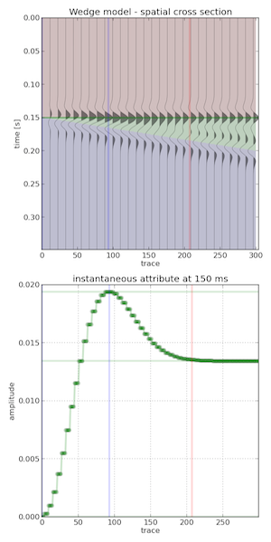
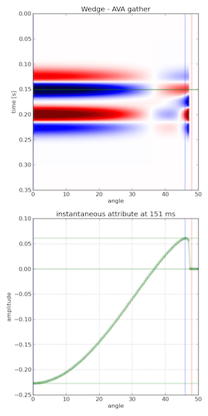
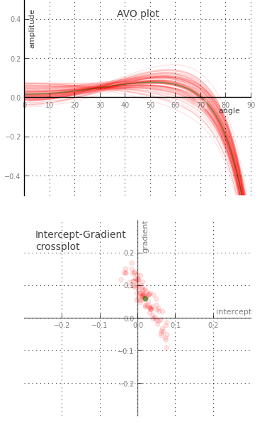
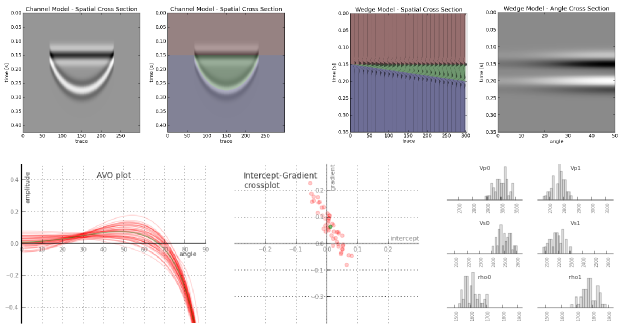
 A wedge model & tuning curve An AVA gather for a Class 4 sand    A stochastic AVA crossplot          

 modelr seismic wedge modelmodelr seismic avo modelmodelr stochastic avo  model

The most important thing nobody does

A couple of weeks ago, we told you we were up to something. Today, we're excited to announce modelr.io — a new seismic forward modeling tool for interpreters and the seismically inclined.

Modelr is a web app, so it runs in the browser, on any device. You don't need permission to try it, and there's never anything to install. No licenses, no dongles, no not being able to run it at home, or on the train.

Later this week, we'll look at some of the things Modelr can do. In the meantime, please have a play with it.
Just go to modelr.io and hit Demo, or click on the screenshot below. If you like what you see, then think about signing up — the more support we get, the faster we can make it into the awesome tool we believe it can be. And tell your friends!

If you're intrigued but unconvinced, sign up for occasional news about Modelr:

This will add you to the email list for the modeling tool. We never share user details with anyone. You can unsubscribe any time.

A long weekend of creative geoscience computing

The Rock Hack is in three weeks. If you're in Houston, for AAPG or otherwise, this is going to be a great opportunity to learn some new computer skills, build some tools, or just get some serious coding done. The Agile guys — me, Evan, and Ben — will be hanging out at START Houston, laptops open, all say 5 and 6 April, about 8:30 till 5. The breakfast burritos and beers are on us.

Unlike the geophysics hackathon last September, this won't be a contest. We're going to try a more relaxed, unstructured event. So don't be shy! If you've always wanted to try building something but don't know where to start, or just want to chat about The Next Big Thing in geoscience or technology — please drop in for an hour, or a day.

Here are some ideas we're kicking around for projects to work on:

  • Sequence stratigraphy calibration app to tie events to absolute geologic time and to help interpret systems tracts.
  • Wireline log 'attributes'.
  • Automatic well-to-well correlation.
  • Facies recognition from core.
  • Automatic photomicrograph interpretation: grain size, porosity, sorting, and so on.
  • A mobile app for finding and capturing data about outcrops.
  • An open source basin modeling tool.

Short course

If you feel like a short course would get you started faster, then come along on Friday 4 April. Evan will be hosting a 1-day course, leading you through getting set up for learning Python, learning some syntax, and getting started on the path to scientific computing. You won't have super-powers by the end of the day, but you'll know how to get them.

Eventbrite - Agile Geocomputing

The course includes food and drink, and lots of code to go off and play with. If you've always wanted to get started programming, this is your chance!

Transforming geology into seismic

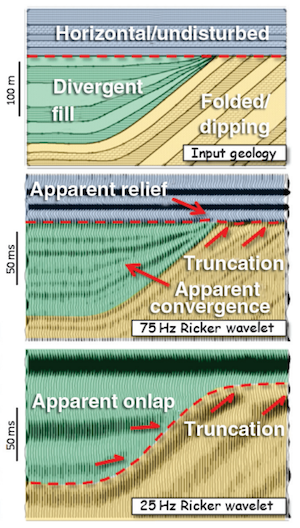
Hart (2013). ©SEG/AAPGForward modeling of seismic data is the most important workflow that nobody does.

Why is it important?

  • Communicate with your team. You know your seismic has a peak frequency of 22 Hz and your target is 15–50 m thick. Modeling can help illustrate the likely resolution limits of your data, and how much better it would be with twice the bandwidth, or half the noise.
  • Calibrate your attributes. Sure, the wells are wet, but what if they had gas in that thick sand? You can predict the effects of changing the lithology, or thickness, or porosity, or anything else, on your seismic data.
  • Calibrate your intuition. Only by predicting the seismic reponse of the geology you think you're dealing with, and comparing this with the response you actually get, can you start to get a feel for what you're really interpreting. Viz Bruce Hart's great review paper we mentioned last year (right).

Why does nobody do it?

Well, not 'nobody'. Most interpreters make 1D forward models — synthetic seismograms — as part of the well tie workflow. Model gathers are common in AVO analysis. But it's very unusual to see other 2D models, and I'm not sure I've ever seen a 3D model outside of an academic environment. Why is this, when there's so much to be gained? I don't know, but I think it has something to do with software.

  • Subsurface software is niche. So vendors are looking at a small group of users for almost any workflow, let alone one that nobody does. So the market isn't very competitive.
  • Modeling workflows aren't rocket surgery, but they are a bit tricky. There's geology, there's signal processing, there's big equations, there's rock physics. Not to mention data wrangling. Who's up for that?
  • Big companies tend to buy one or two licenses of niche software, because it tends to be expensive and there are software committees and gatekeepers to negotiate with. So no-one who needs it has access to it. So you give up and go back to drawing wedges and wavelets in PowerPoint.

Okay, I get it, how is this helping?

We've been busy lately building something we hope will help. We're really, really excited about it. It's on the web, so it runs on any device. It doesn't cost thousands of dollars. And it makes forward models...

That's all I'm saying for now. To be the first to hear when it's out, sign up for news here:

This will add you to the email list for the modeling tool. We never share user details with anyone. You can unsubscribe any time.

Seismic models: Hart, BS (2013). Whither seismic stratigraphy? Interpretation, volume 1 (1). The image is copyright of SEG and AAPG.

Rock Hack 2014

We're hosting another hackathon! This time, we're inviting geologists in all their colourful guises to come and help dream up cool tools, find new datasets, and build useful stuff. Mark your calendar: 5 & 6 April, right before AAPG.

On 4 April there's the added fun of a Creative geocomputing course. So you can learn some skills, then put them into practice right away. More on the course next week.

What's a hackathon?

It's not as scary — or as illegal — as it sounds! And it's not just for coders. It's just a roomful of creative geologists and friendly programmers figuring out two things together:

  1. What tools would help us in our work?
  2. How can we build those tools?

So for example, we might think about problems like these:

  • A sequence stratigraphy calibration app to tie events to absolute geologic time
  • Wireline log 'attributes'
  • Automatic well-to-well correlation
  • Facies recognition from core
  • Automatic photomicrograph interpretation: grain size, porosity, sorting, and so on
  • A mobile app for finding and capturing data about outcrops
  • Sedimentation rate analysis, accounting for unconformities, compaction, and grain size

I bet you can think of something you'd like to build — add it to the list!

Still not sure? Check out what we did at the Geophysics Hackathon last autumn...

How do I sign up?

You can sign up for the creative geocomputing course at Eventbrite.

If you think Rock Hack sounds like a fun way to spend a weekend, please drop us a line or sign up at Hacker League. If you're not sure, please come anyway! We love visitors.

If you think you know someone who'd be up for it, let them know with the sharing buttons below.

The poster image is from an original work by Flickr user selkovjr.

Free software tips

Open source software is often called 'free' software. 'Free as in freedom, not free as in beer', goes the slogan (undoubtedly a strange way to put it, since beer is rarely free). But something we must not forget about free and open software: someone, a human, had to build it.

It's not just open source software — a lot of stuff is free to use these days. Here are a few of the things I use regularly that are free:

Wow. That list was easy to write; I bet I've barely scratched the surface.

It's clear that some of this stuff is not free, strictly speaking. The adage 'if you're not paying for it, then you're the product' is often true — Google places ads in my Gmail web view, Facebook is similarly ad driven, your LinkedIn account provides valuable data and a prospect to paying members, mostly in human resources. 

But it's also clear that a few individuals in the world are creating massive, almost unmeasurable (if you think about Linux or Wikipedia), value in the world... and then giving it away. Think about that. Think about what that enables in the world. It's remarkable, especially when I think about all the physical junk I pay for. 

Give something back

I won't pretend to be consistent or rigorous about this, but since I started Agile I've tried to pay people for the awesome things that I use every day. I donate to Wikimedia, Mozilla and Creative Commons, I pay for the (free) Ubuntu Linux distribution, I buy the paid version of apps, and I buy the basic level of freemium apps rather than using the free one. If some freeware helps me, I send the developer $25 (or whatever) via PayPal.

I wonder how many corporations donate to Wikipedia to reflect the huge contribution it makes to their employees' ability to perform their work? How would it compare with how much it spends on tipping restaurant servers and cab drivers every year in the US, even when the service was mediocre?

There are lots of ways for developers and other creators to get paid for work they might otherwise have done for free, or at great personal expense or risk. For example, Kickstarter and Indiegogo are popular crowdfunding platforms. And I recently read about a Drupal developer's success with Gittip, a new tipping protocol.

Next time you get real value from something that cost you nothing, think about supporting the human being that put it together. 

The image is CC-BY-SA and created by Wikimedia Commons user JIP.

To make up microseismic

I am not a proponent of making up fictitious data, but for the purposes of demonstrating technology, why not? This post is the third in a three-part follow-up from the private beta I did in Calgary a few weeks ago. You can check out the IPython Notebook version too. If you want more of this in person, sign up at the bottom or drop us a line. We want these examples to be easily readable, especially if you aren't a coder, so please let us know how we are doing.

Start by importing some packages that you'll need into the workspace,

%pylab inline
import numpy as np
from scipy.interpolate import splprep, splev
import matplotlib.pyplot as plt
import mayavi.mlab as mplt
from mpl_toolkits.mplot3d import Axes3D

Define a borehole path

We define the trajectory of a borehole, using a series of x, y, z points, and make each component of the borehole an array. If we had a real well, we load the numbers from the deviation survey just the same.

trajectory = np.array([[   0,   0,    0],
                       [   0,   0, -100],
                       [   0,   0, -200],
                       [   5,   0, -300],
                       [  10,  10, -400],
                       [  20,  20, -500],
                       [  40,  80, -650],
                       [ 160, 160, -700],
                       [ 600, 400, -800],
                       [1500, 960, -800]])
x = trajectory[:,0]
y = trajectory[:,1]
z = trajectory[:,2]

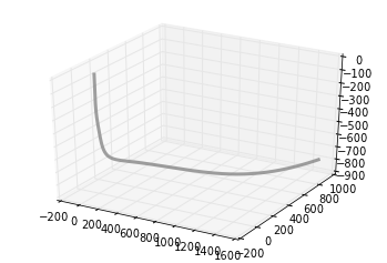
But since we want the borehole to be continuous and smoothly shaped, we can up-sample the borehole by finding the B-spline representation of the well path,

smoothness = 3.0
spline_order = 3
nest = -1 # estimate of number of knots needed (-1 = maximal)
knot_points, u = splprep([x,y,z], s=smoothness, k=spline_order, nest=-1)

# Evaluate spline, including interpolated points
x_int, y_int, z_int = splev(np.linspace(0, 1, 400), knot_points)

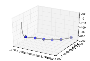
plt.gca(projection='3d')
plt.plot(x_int, y_int, z_int, color='grey', lw=3, alpha=0.75)
plt.show()

Define frac ports

Let's define a completion program so that our wellbore has 6 frac stages,

number_of_fracs = 6

and let's make it so that each one emanates from equally spaced frac ports spanning the bottom two-thirds of the well.

x_frac, y_frac, z_frac = splev(np.linspace(0.33, 1, number_of_fracs), knot_points)

Make a set of 3D axes, so we can plot the well path and the frac ports.

ax = plt.axes(projection='3d')
ax.plot(x_int, y_int, z_int, color='grey',
        lw=3, alpha=0.75)
ax.scatter(x_frac, y_frac, z_frac,
        s=100, c='grey')
plt.show()

Set a colour for each stage by cycling through red, green, and blue,

stage_color = []
for i in np.arange(number_of_fracs):
    color = (1.0, 0.1, 0.1)
    stage_color.append(np.roll(color, i))
stage_color = tuple(map(tuple, stage_color))

Define microseismic points

One approach is to create some dimensions for each frac stage and generate 100 points randomly within each zone. Each frac has an x half-length, y half-length, and z half-length. Let's also vary these randomly for each of the 6 stages. Define the dimensions for each stage:

frac_dims = []
half_extents = [500, 1000, 250]
for i in range(number_of_fracs):
    for j in range(len(half_extents)):
        dim = np.random.rand(3)[j] * half_extents[j]
        frac_dims.append(dim)  
frac_dims = np.reshape(frac_dims, (number_of_fracs, 3))

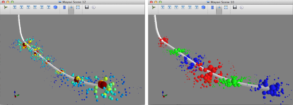
Plot microseismic point clouds with 100 points for each stage. The following code should launch a 3D viewer scene in its own window:

size_scalar = 100000
mplt.plot3d(x_int, y_int, z_int, tube_radius=10)
for i in range(number_of_fracs):
    x_cloud = frac_dims[i,0] * (np.random.rand(100) - 0.5)
    y_cloud = frac_dims[i,1] * (np.random.rand(100) - 0.5)
    z_cloud = frac_dims[i,2] * (np.random.rand(100) - 0.5)

    x_event = x_frac[i] + x_cloud
    y_event = y_frac[i] + y_cloud     
    z_event = z_frac[i] + z_cloud
    
    # Let's make the size of each point inversely proportional 
    # to the distance from the frac port
    size = size_scalar / ((x_cloud**2 + y_cloud**2 + z_cloud**2)**0.002)
    
    mplt.points3d(x_event, y_event, z_event, size, mode='sphere', colormap='jet')

You can swap out the last line in the code block above with mplt.points3d(x_event, y_event, z_event, size, mode='sphere', color=stage_color[i]) to colour each event by its corresponding stage.

A day of geocomputing

I will be in Calgary in the new year and running a one-day version of this new course. To start building your own tools, pick a date and sign up:

Eventbrite - Agile Geocomputing    Eventbrite - Agile Geocomputing

To make a wedge

We'll need a wavelet like the one we made last time. We could import it, if we've made one, but SciPy also has one so we can save ourselves the trouble. Remember to put %pylab inline at the top if using IPython notebook.

import numpy as np
from scipy.signal import ricker
import matplotlib.pyplot as plt

Now we need to make a physical earth model with three rock layers. In this example, let's make an acoustic impedance earth model. To keep it simple, let's define the earth model with two-way-travel time along the vertical axis (as opposed to depth). There are number of ways you could describe a wedge using math, and you could probably come up with a way that is better than mine. Here's a way:

nsamps, ntraces = [600, 500]
rock_names = ['shale 1', 'sand', 'shale 2']
rock_grid = np.zeros((n_samples, n_traces))

def make_wedge(n_samples, n_traces, layer_1_thickness, start_wedge, end_wedge):
    for j in np.arange(n_traces): 
        for i in np.arange(n_samples):      
            if i <= layer_1_thickness:      
rock_grid[i][j] = 1 if i > layer_1_thickness:
rock_grid[i][j] = 3 if j >= start_wedge and i - layer_1_thickness < j-start_wedge:
rock_grid[i][j] = 2 if j >= end_wedge and i > layer_1_thickness+(end_wedge-start_wedge):
rock_grid[i][j] = 3 return rock_grid

Let's insert some numbers into our wedge function and make a particular geometry.

layer_1_thickness = 200
start_wedge = 50
end_wedge = 250
rock_grid = make_wedge(n_samples, n_traces, 
            layer_1_thickness, start_wedge, 
            end_wedge)

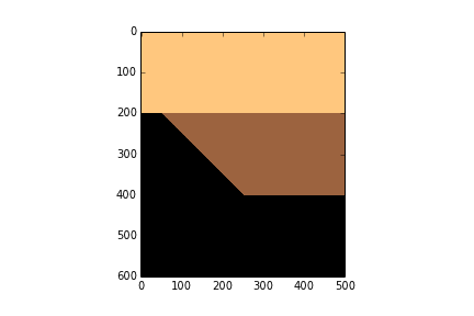
plt.imshow(rock_grid, cmap='copper_r')

Now we can give each layer in the wedge properties.

vp = np.array([3300., 3200., 3300.]) 
rho = np.array([2600., 2550., 2650.]) 
AI = vp*rho
AI = AI / 10e6 # re-scale (optional step)

Then assign values assign them accordingly to every sample in the rock model.

model = np.copy(rock_grid)
model[rock_grid == 1] = AI[0]
model[rock_grid == 2] = AI[1]
model[rock_grid == 3] = AI[2]
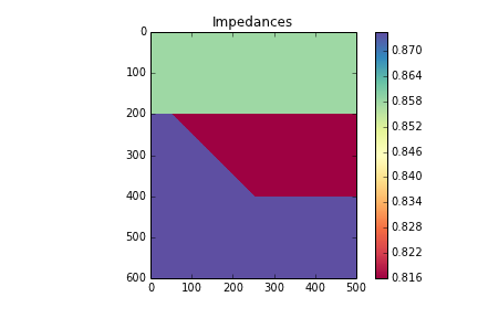
plt.imshow(model, cmap='Spectral')
plt.colorbar()
plt.title('Impedances')

Now we can compute the reflection coefficients. I have left out a plot of the reflection coefficients, but you can check it out in the full version in the nbviewer

upper = model[:-1][:]
lower = model[1:][:]
rc = (lower - upper) / (lower + upper)
maxrc = abs(np.amax(rc))

Now we make the wavelet interact with the model using convolution. The convolution function already exists in the SciPy signal library, so we can just import it.

from scipy.signal import convolve
def make_synth(f):
    synth = np.zeros((n_samples+len(t)-2, n_traces))
    wavelet = ricker(512, 1e3/(4.*f))
    wavelet = wavelet / max(wavelet)   # normalize
    for k in range(n_traces):
        synth[:,k] = convolve(rc[:,k], wavelet)
    synth = synth[ np.ceil(len(wavelet))/2 : -np.ceil(len(wavelet))/2, : ]
    return synth

Finally, we plot the results.

frequencies = array([5, 10, 15]) plt.figure(figsize = (15, 4)) for i in np.arange(len(frequencies)): this_plot = make_synth(frequencies[i]) plt.subplot(1, len(frequencies), i+1) plt.imshow(this_plot, cmap='RdBu', vmax=maxrc, vmin=-maxrc, aspect=1) plt.title( '%d Hz wavelet' % freqs[i] ) plt.grid() plt.axis('tight') # Add some labels for i, names in enumerate(rock_names): plt.text(400, 100+((end_wedge-start_wedge)*i+1), names, fontsize=14, color='gray', horizontalalignment='center', verticalalignment='center')


That's it. As you can see, the marriage of building mathematical functions and plotting them can be a really powerful tool you can apply to almost any physical problem you happen to find yourself working on.

You can access the full version in the nbviewer. It has a few more figures than what is shown in this post.

A day of geocomputing

I will be in Calgary in the new year and running a one-day version of this new course. To start building your own tools, pick a date and sign up:

Eventbrite - Agile Geocomputing    Eventbrite - Agile Geocomputing

The developer's mind

Humbled by the aura of the legendary Cavendish Labs sitting in the adjacent building next door, I refrain from expressing the full extent of my awe and reverence for this special place. "Sure", I think, "it's no big deal. Let's get on with it". I came to Cambridge to collaborate with Pietro Berkes. He's building Canopy Geo at Enthought. We spent the day spiking, apparently. Working shoulder to shoulder with Pietro was nearly as responsive as dictating a vision to a painter and watching it emerge before my eyes. He's darn good. During my visit, I took notice of some characteristics and guiding principles that top developers, such as himself and his colleagues, bring to their work.

On whiteboarding

The best way to be understood, to connect, or to teach, is to do it one-on-one in front of a whiteboard. It is fitting that all of the walls of their office space are whiteboard walls. Old marks wiped clean but still visible show remnant algorithms sketched out and stacked up upon each other. A well-worn workshop, where writing on the walls is the cultural norm. And for electronic communication? Some are deliberate to only check emails three times a day: first thing in the morning, midday, and mid afternoon. Any more often, would be disruptive to their flow. Email is the enemy of real work, but instant messaging can be be a good productivity tool. 

On discipline

To build something that is extensible takes a good deal of thoughfulness and discipline. Code will survive long after the project is over and the programmer has moved on. This doesn't just mean leaving an adequate documentation trail behind you, but also building a solid foundation that others can contribute to. Being Agile, it turns out, although not the only choice, also takes discipline and diligence in order to be effective. 

On ownership and responsibilty 

Authority is not given, responsibility is taken. Many of the best developers define themselves by the authorship of code and libraries. So attribution is not only necessary politeness, it is a direct line of communication. What body of work would you stand up and speak for? Someone may find a bug at 9:00 am in a different time zone. Will they wait till 2:00 pm to hear from you? Somehow, this decentralized system of self-appointed responsibilty just works. The longevity of emotional and intellectual labour, particuarly in an open source setting, is a fascinating concept. The work becomes more relevant because the developer never stops caring for it. You can change projects, you can change languages, you can change companies, but your work never leaves you. If that notion excites you, you are making an impact. 

The developer knows that prowess is earned by execution. They thrive in an accepted sub-culture of meritocracy: largely free of politics, organizational hierarchies, and other social drama that get in the way of the real work. With a mind cleared to deal with essential tasks, what emerges is the ego of an artist and a creator with the potential to act on it. "Now that we can build anything, what do we do next?"