A forensic audit of seismic data

The SEG-Y “standard” is famously non-standard. (Those air quotes are actually part of the “standard”.)

For example, the inline and crossline location of a given trace — two things that you must have in order to load the data vaguely properly — are “recommended” (remember, it’s a “standard”) to be given in the trace’s header, at byte locations 189 and 193 respectively. Indeed, they might well be there. Or 1 and 5 (well, 5 or 9). Or somewhere else. Or not there at all.

Don Robinson at Resolve told me recently that he has seen more than 180 byte-location combinations, and he said another service company had seen more than 300.

All this can make loading seismic data really, really annoying.

I’d like to propose that the community performs a kind of forensic audit of SEG-Y files. I have 5 main questions:

  1. What proportion of files claim to be Rev 0, Rev 1, and Rev 2? And what standard are they actually? (If any!)

  2. What proportion of files in the wild use IBM vs IEEE floats? What about integers?

  3. What proportion of files in the wild use little-endian vs big-endian byte order. (Please tell me there's no middle-endian data out there!)

  4. What proportion of files in the wild use EBCDIC vs ASCII encoded textual file headers? (Again, I would hope there are no other encodings in use, but I bet there are.)

  5. What proportion of files use the Strongly recommended and Recommended byte locations for trace numbers, sample counts, sample interval, coordinates and inline–crossline numbers?

For each of these <things> it would also be interesting to know:

  • How does <thing> vary with the other things? That is, what's the cross-correlation matrix?

  • How does <thing> vary with the age of the file? Is there a temporal trend?

  • How does <thing> vary with the provenance of the file? What's the geographic trend? (For example, Don told me that the prevalence of PC-based interpretation packages in Canada led to widespread early adoption of IEEE floats and little-endian byte order; indeed, he says that 90% of the SEG-Y he sees in the wild is still IBM ormatted floats!)

While we’re at it, I'd also like in some more esoteric things:

  • How many files have cornerpoints in the text header, and/or trace locations in trace headers?

  • How many files have an unambiguous CRS in the text header?

  • How many files have information about the processing sequence in the text header? (E.g. imaging details, filters, etc.)

  • How many files have incorrect information in the headers (e.g. locations, sample interval, byte format, etc)

  • How many processors bother putting useful things like elevation, filters, sweeps, fold at target, etc, in the trace headers?

I don’t quite know how such a survey would happen. Most of these things are obviously detectable from the files themselves. Perhaps some of the many seismic data management systems already track these things. Or maybe you’re a data manager and you have some anecdotal data you can share.

What do you think? I’d love to hear your thoughts in the comments. Maybe there’s a good hackathon project here!

All the wedges

Wedges are a staple of the seismic interpreter’s diet. These simple little models show at a glance how two seismic reflections interact with each other when a rock layer thins down to — and below — the resolution limit of the data. We can also easily study how the interaction changes as we vary the wavelet’s properties, especially its frequency content.

Here’s how to make and plot a basic wedge model with Python in the latest version of bruges, v0.4.2:

 
import bruges as bg
import matplotlib.pyplot as plt

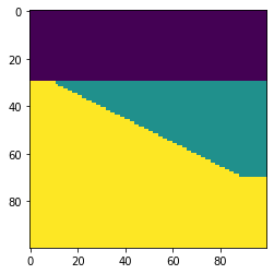
wedge, *_ = bg.models.wedge()

plt.imshow(wedge)
wedge_basic.png

It really is that simple! This model is rather simplistic though: it contains no stratigraphy, and the numerical content of the 2D array is just a bunch of integers. Let’s instead make a P-wave velocity model, with an internal bed of faster rock inside the wedge:

 
strat = [2.35, (2.40, 2.50, 2.40), 2.65]
wedge, *_ = bg.models.wedge(strat=strat)

plt.imshow(wedge)
plt.colorbar()
wedge_layer.png

We can also choose to make the internal geometry top- or bottom-conformant, mimicking onlap or an unconformity, respectively.

 
strat = strat=[0, 7*[1,2], 3]
wedge, *_ = bg.models.wedge(strat=strat,
                            conformance='base'
                           )

plt.imshow(wedge)
wedge_unconformity.png

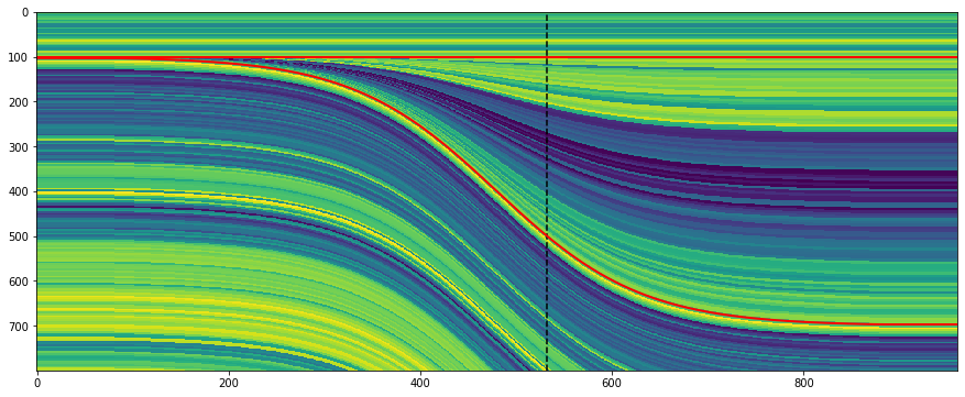
The killer feature of this new function might be using a log to make the stratigraphy, rather than just a few beds. This is straightforward to do with welly, because it makes selecting depth intervals and resampling a bit easier:

 
import welly

gr = welly.Well.from_las('R-39.las').data['GR']
log_above = gr.to_basis(stop=2620, step=1.0)
log_wedge = gr.to_basis(start=2620, stop=2720, step=1.0)
log_below = gr.to_basis(start=2720, step=1.0)

strat = (log_above, log_wedge, log_below)
depth, width = (100, 400, 100), (40, 200, 40)
wedge, top, base, ref = bg.models.wedge(depth=depth,
                                        width=width,
                                        strat=strat,
                                        thickness=(0, 1.5)
                                       )

plt.figure(figsize=(15, 6))
plt.imshow(wedge, aspect='auto')
plt.axvline(ref, color='k', ls='--')
plt.plot(top, 'r', lw=2)
plt.plot(base, 'r', lw=2)
wedge_log.png

Notice that the function returns to you the top and base of the wedgy part, as well as the position of the ‘reference’, in this case the well.

I’m not sure if anyone wanted this feature… but you can make clinoform models too:

wedge_log_clino.png

Lastly, the whole point of all this was to make a synthetic — the forward model of the seismic experiment. We can make a convolutional model with just a few more lines of code:

 
strat = np.array([2.32 * 2.65,  # Layer 1
                  2.35 * 2.60,  # Layer 2
                  2.35 * 2.62,  # Layer 3
                 ])

# Fancy indexing into the rocks with the model.
wedge, top, base, ref = bg.models.wedge(strat=strat)

# Make reflectivity.
rc = (wedge[1:] - wedge[:-1]) / (wedge[1:] + wedge[:-1])

# Get a wavelet.
ricker = bg.filters.ricker(0.064, 0.001, 40)

# Repeated 1D convolution for a synthetic.
syn = np.apply_along_axis(np.convolve, arr=rc, axis=0, v=ricker, mode='same')
wedge_synthetic.png

That covers most of what the tool can do — for now. I’m working on extending the models to three dimensions, so you will be able to vary layers or rock properties in the 3rd dimension. In the meantime, take these wedges for a spin and see what you can make! Do share your models on Twitter or LinkedIn, and have fun!

Which open licence should I choose?

I’ve written about open data a few times recently. And not-so-recently. And there’s been quite a bit of chat about open subsurface benchmarks in the Software Underground recently. As more people consider openly releasing data — or code, or other content — one question comes up fairly often is: Which licence should I choose?

I’ll start at the beginning, and I am not a lawyer, but this is going to be very high level. So do click on the links to read more.

What is copyright?

You automatically own the copyright to anything original that you create. You don’t have to register it, but the thing you made — and it must be a thing, you can’t copyright ideas — must be original. It could be a photo, a song, or a seismic interpretation. Physical measurements with no creative input, such as well logs, are not copyrightable… but a database consisting of such data is (so-called database rights). Your rights are exclusive, worldwide, and last until some years after you die (it varies).

If someone wants to use your work, even if they just found it on the Internet, they must either claim Fair Use, or seek permission from you. Giving permission means granting a licence; it can be as restrictive and arcane as you want.

If you don’t want people bothering you about licences, or if you want to actively encourage people to use and adapt your work, you can preemptively grant an open licence.

What is openness?

Before you start thinking about licences, there are two more big things to learn about:

  1. What is open? Not all licences, not even all Creative Commons licences, meet the Open Definition. In brief, this states that “Open data and content can be freely used, modified, and shared by anyone for any purpose” — you can’t restrict people based on their use case or location. So licences that forbid commercial application are not open.

  2. What is permissiveness? Once you’ve decided to go open, you need to decide where you stand on permissiveness. Some licences, notably those advocated by the GNU Free Software Movement, compel licensees (users) to preserve the openness of the work in any future redistribution. This ‘viral’ condition is sometimes called copyleft.

In some circles, a near-religious war smoulders on the permissiveness issue. You need to make up your own mind where you stand, or at least understand the issues.

By the way, granting a licence does not mean giving up your rights. In fact, you must own the copyright in order to grant the licence. Many scientists don’t realize we’ve been giving away the copyright in our work for decades, as a (completely unnecessary and made up) condition of publication.

Another source of confusion: open licences are also not the same thing as public domain. Public domain means that the work is free from copyright restrictions. In general though, it cannot be applied to a copyrighted work (though CC0 tries to relinquish copyright where possible). For example, On The Origin of Species is public domain, as is most work produced by the United States government (for example, by the USGS).

One last thing: an often overlooked aspect of licensing is protection for you, the licensor. All common licences include language that indemnifies you from misuse or misinterpretation of your work. So be careful about putting your stuff ‘out there’ with anything other than a standard licence: you may be leaving yourself open to liability issues later.

Open licences

Rather than writing a lot of stuff that’s been written by smarter people than me, I thought I’d draw a diagram to try to explain the differences between some common licences (there are certainly a lot more than the ones I mention here).

Just to re-iterate: there are a lot more licences than the ones mentioned here, these are just examples.

What do I recommend?

For content, my personal belief is that CC-BY most aptly captures the way science works. Scientists 'build on the shoulders of giants' by re-using the work of others with fastidious attribution, usually by citation. Accordingly, the CC-BY protects the licensor, ensures attribution, and that's it. If you prefer copyleft licences, the equivalent licence is CC-BY-SA.

But Creative Commons recommend against using CC licences for source code, so what should you do then?

For code, the permissive licence closest to CC-BY is the MIT/BSD/Apache family of licences, of which only the Apache 2.0 licence offers some specific protections with respect to patents (in particular, it protects licensees from ‘upstream’ patent infringements). The equivalent copyleft licences are the GPL (for applications) and LGPL (for libraries).

For data, I tend to use CC-BY, but there are some specialist data licences (beware, they are poorly named in my opinion: the seemingly ‘vanilla’ ODbL is copyleft; the permissive equivalent is ODC-By).

What about mixed content, like a Jupyter Notebook? You have to be practical; maybe it depends on whether you consider your notebooks to be 'content' or 'source code'. I sometimes put at the bottom of a notebook something like Open source content. Text is CC-BY, code is Apache 2.0 and I think this makes my intent clear.

Tools

There are some tools around to help you make a choice of licence:

Last thing

Note that open licences are just one piece of the jigsaw puzzle of reproducible science and reusable content. You also need to think about open and accessible data formats (e.g. CSV not XLS), accessible content (DOIs and open indexes), and documentation.

Although insufficient, open licences are a necessary component though. And while licences can be changed, they cannot be revoked… so it’s worth putting some thought into your choices before you start pushing your content out into the world.

If it seems hard to navigate, do get in touch, we’d be happy to help if and where we can (notwithstadning IANAL). If your situation is at all complicated I recommend seeking professional legal advice — but do go out of your way to find one who understands both the motivation for, and the legal issues around, open licensing.

The procedural generation of geology

Procedural generation is a way of faking stuff with computers. But by writing code, or otherwise defining algorithms — not by manually choosing or composing or sculpting things. It’s used to produce landscapes and other assets in computer games, or just to make beautiful things. Honestly, I know almost nothing about it, and I don’t play computer games, so I’m really just coming at it from the ‘beautiful things’ side. So let’s just stick to looking at some examples…

Robert Hodgin produces jaw-dropping images, and happily one of his favourite subjects is meandering rivers. Better yet, Harold Fisk’s maps are among his inspirations. The results are mindblowing — just check this animation out:

What’s really remarkable is that everything on that map is procedurally generated: the roadways, the vegetation, the wonderful names.

If you love meanders (who doesn’t love meanders?), then you also need to know about Zoltan Sylvester’s work (not to mention his Etsy store). He produces some great animations, and also maintains some open-source Python projects (e.g. meanderpy) for producing them, so you can get stuck in and make your own.

It’s not just about meanders. Artist Tyler Hobbs has produced some striking images that strongly resemble structural cross-sections. In this thread he mentions that this wasn’t his goal, they just came out that way.

Mattias Herder, a space-obsessed viz wizard, did intend to produce crystals though. He’s using Houdini software, which I believe is also what Robert Hodgin uses for his maps. I wonder if any geologists are using it…

Landscapes are one of the big areas of application of this sort of tech, and while not strictly geological, I love these frozen vistas by French artist Guillaume Cottet:

Finally, this example from digital artist Ian Smith hints at a bit of the creative process. This guy really knows how to make rocks…

This is all so much magic to me, but I’m intrigued. Like the black hole in Interstellar, could this kind of work actually shed light on how dynamic, non-linear natural systems work? Or is it just an illusion?

What is an Ormsby wavelet anyway?

If you dabble in reflection seismic analysis, you probably know the Ricker wavelet. We’ve visited it a few times on this blog — Evan once showed how to make and plot one, I looked at some analytic properties of it, and we even played golf with it.

The Ricker is everywhere, but it has an important limitation — bandwidth. Its shape in the frequency domain is roughly Gaussian (below, left), which is the reason it only really has one parameter: the central frequency. This kind of spectrum is sometimes okay for older seismic surveys, especially marine data, because it matches the bandwidth reasonably. But for modern surveys, or even old land data, we often want a broader set of frequencies — more of a trapezoidal spectral shape. We need the Ormsby wavelet:

ricker-vs-ormsby.png

How to make an Ormsby wavelet

The earliest reference I can find to the Ormsby wavelet is in an article by Harold Ryan entitled, Ricker, Ormsby, Klauder, Butterworth — a choice of wavelets, in the September 1994 issue of the CSEG Recorder. It’s not clear at all who Ormsby was, other than “an aeronautical engineer”. And I don’t think anyone outside exploration geophysics knows what an Ormsby is, they just call it a ‘bandpass filter’.

Ryan helpfully provided both a time-domain analytic expression — which turns out to have four typos use the classical definiton of the sinc function — and a plot:

The equation in Ryan, and my modified Figure 3 (right). the result of the equation is in red.

The equation in Ryan, and my modified Figure 3 (right). the result of the equation is in red.

ryan_ormsby-cf-expression-2.png

This equation does not produce the wavelet (black) in the plot, however, it produces the one I’ve added in red. If you find this surprising, you shouldn’t — in my experience, it’s very common for the words and/or maths in a paper not to match its figures. [Edit: as noted above, in this case it’s because of how NumPy’s sinc function is defined; see the comment from Robert Kern, below.] We established this at the SEG Repro Zoo in 2018. If an author is not required to produce code or data, it’s not very surprising; and even if they do, the peer review system is not set up for referees to do this kind of check — apart from anything else, it’s far too onerous. But I digress.

After some fiddling around, I realized that the expression being passed to NumPy’s sinc function should be \(ft\), not \(\pi ft\). This produces a result that matches the figure almost exactly (and, counting wiggles, has the right frequency). So here’s the result of that new expression, shown in green here with the original figure (black) and the same red wavelet as above:

ryan_ormsby-cf-bruges.png

This green thing is the wavelet implemented in bruges so it’s easy to produce it; the arguments are the duration (0.4 seconds), the sample interval dt (4 ms) and the corner frequencies f (5, 10, 40, and 45 Hz respectively):

bruges.filters.ormsby(duration=0.4, dt=0.004, f=[5, 10, 40, 45])

What about other examples from the literature?

Good question! Apart from my own Python code in bruges, I did find one or two other implementations:

So it seems from this tiny experiment that only one of the implementations I found matched the figure in the Ryan article perfectly. The other wavelets are variations on the theme. Which is probably fine — after all, they are all only models for real seismic impulses — but in the interests of scientific reproducibility, I think it underscores the importance of transparent methodology and publishing your code.


Update on 9 Feb: A conversation in Software Underground revealed that Petrel’s version of the Ormsby wavelet matches the bruges implementation — but with a triangular window multiplied in (similar to how a Hamming window is multiplied into the seismic.jl version.


518px-Jupyter_logo.svg.png

I pushed my Python Jupyter Notebook to the new repro-zoo repository on GitHub. Please feel free to fork this project and add your own attempted reproductions of computational geoscience papers.

The original repro-zoo repo from the 2018 event is on SEG’s GitHub.


References

Ryan, H (1994). Ricker, Ormsby, Klauder, Butterworth — a choice of wavelets. CSEG Recorder 19 (7). Available online.

Soo-Kyung Miong, Robert R. Stewart and Joe Wong (2007). Characterizing the near surface with VSP and well logs. CREWES Research Report 19. Available online.

Does your machine learning smell?

Martin Fowler and Kent Beck popularized the term ‘code smell’ in the book Refactoring. They were describing the subtle signs of deeper trouble in code — signs that a program’s source code might need refactoring (restructuring and rewriting). There are too many aromas to list here, but here are some examples (remember, these things are not necessarily problems in themselves, but they suggest you need to look more closely):

  • Duplicated code.

  • Contrived complexity (also known as showing off).

  • Functions with many arguments, suggesting overwork.

  • Very long functions, which are hard to read.

More recently, data scientist Felienne Hermans applied the principle to the world’s number one programming environment: spreadsheets. The statistics on spreadsheet bugs are quite worrying, and Hermans enumerated the smells that might lead you to them. Here are four of her original five ‘formula’ smells, notice how they correspond to the code smells above:

  • Duplicated formulas.

  • Conditional complexity (e.g. nested IF statements).

  • Multiple references, analogous to the ‘many arguments’ smell.

  • Multiple operations in one cell.

What does a machine learning project smell like?

Most machine learning projects are code projects, so some familiar smells might be emanating from the codebase (if we even have access to it). But machine learning models are themselves functions — machines that map input X to some target y. And even if the statistical model is simple, like a KNN classifier, the workflow is a sort of ‘metamodel’ and can have complexities of its own. So what are the ‘ML smells’ that might alert us to deeper problems in our prediction tools?

I asked this question on Twitter (below) and in the Software Underground

I got some great responses. Here are some ideas adapted from them, with due credit to the people named:

  • Very high accuracy, especially a complex model on a novel task. (Ari Hartikainen, Helsinki and Lukas Mosser, Athens; both mentioned numbers around 0.99 but on earth science problems I start to get suspicious well before that: anything over 0.7 is excellent, and anything over 0.8 suggests ‘special efforts’ have been made.)

  • Excessive precision on hyperparameters might suggest over-tuning. (Chris Dinneen, Perth)

  • Counterintuitive model weights, e.g. known effects have low feature importance. (Reece Hopkins, Anchorage)

  • Unreproducible, non-deterministic code, e.g. not setting random seeds. (Reece Hopkins again)

  • No description of the train–val–test split, or justification for how it was done. Leakage between training and blind data is easy to introduce with random splits in spatially correlated data. (Justin Gosses, Houston)

  • No discussion of ground truth and how the target labels relate to it. (Justin Gosses again)

  • Less than 80% of the effort spent on preparing the data. (Michael Pyrcz, Austin — who actually said 90%)

  • No discussion of the evaluation metric, eg how it was selected or designed (Dan Buscombe, Flagstaff)

  • No consideration of the precision–recall trade-off, especially in a binary classification task. (Dan Buscombe again)

  • Strong class imbalance and no explicit mention of how it was handled. (Dan Buscombe again)

  • Skewed feature importance (on one or two features) might suggest feature leakage. (John Ramey, Austin)

  • Excuses, excuses — “we need more data”, “the labels are bad”, etc. (Hallgrim Ludvigsen, Stavanger)

  • AutoML, e.g. using a black box service, or an exhaustive automated seach of models and hyperparameters.

That’s already a long list, but I’m sure there are others. Or perhaps some of these are really the same thing, or are at least connected. What do you think? What red — or at least yellow — flags do you look out for when reviewing machine learning projects? Let us know in the comments below.


If you enjoyed this post, check out the Machine learning project review checklist I wrote bout last year. I’m currently working on a new version of the checklist that includes some tips for things to look for when going over the checklist. Stay tuned for that.


The thumbnail for this post was generated automatically from text (something like, “a robot smelling a flower”… but I made so many I can’t remember exactly!). Like a lot of unconstrained image generation by AI’s, it’s not great, but I quite like it all the same.

The AI is LXMERT from the Allen Institute. Try it out or read the paper.

download (7).png

x lines of Python: static basemaps with contextily

Difficulty rating: Beginner

Something that is often useful in planning is to have a basemap of the area in which you have data or an interest. This can be made using a number of different tools, up to and including full-fledged GIS software, but we will use Contextily for a quick static basemap using Python. Installation is as simple as using conda install contextily or pip install contextily.

The steps that we want to take are the following, expressed in plain English, each of which will roughly be one line of code:

  1. Get a source for our basemap (placenames and similar things)
  2. Get a source for our geological map
  3. Get the location that we would like to map
  4. Plot the location with our geological data
  5. Add the basemap to our geological map
  6. Add the attribution for both maps
  7. Plot our final map

We will start with the imports, which as usual do not count:

 
import contextily as ctx
import matplotlib.pyplot as plt

Contextily has a number of built-in providers of map tiles, which can be accessed using the ctx.providers dictionary. This is nested, with some providers offering multiple tiles. An example is the ctx.providers.OpenStreetMap.Mapnik provider, which contains the following:

 
{'url': 'https://{s}.tile.openstreetmap.org/{z}/{x}/{y}.png',
 'max_zoom': 19,
 'attribution': '(C) OpenStreetMap contributors',
 'name': 'OpenStreetMap.Mapnik'}

The most important parameter in the dictionary for each provider is the url. These are of the form example.com/{z}/{x}/{y}.png. The {z} is the zoom level, while {x} and {y} relate to the latitude and longitude of a given tile, respectively. Note that these are the same as those used by interactive Slippy maps; contextily just downloads them as a single static image.

The easiest is to use one of these providers, but we can also define our own provider, using the above pattern for the URL. For geological data, the Macrostrat project is a great resource, especially because they have a tileserver supplying some detail. Their tileserver can be added using

 
geology_tiles = 'https://tiles.macrostrat.org/carto/{z}/{x}/{y}.png'

We also need a place to map. Contextily has a geocoder that can return the tiles covering a given location. It uses OpenStreetMap, so anything that is present there is useable as a location. This includes countries (e.g. 'Paraguay'), provinces/states ('Nova Scotia'), cities ('Lubumbashi'), and so on.

We will use Nova Scotia as our area of interest, as well as giving our desired map tiles. We can also use .plot() on the Place object to get a look at it immediately, using that basemap.

 
ctx.Place('Nova Scotia', source=ctx.providers.CartoDB.Positron).plot()
The Positron style from Carto for Nova Scotia.

The Positron style from Carto for Nova Scotia.

We'll use a different basemap though:

 
basemap = ctx.providers.Stamen.Toner

We can create the Place with our desired source — geology_tiles in this case — and then plot this on the basemap with some transparency. We will also add an attribution, since we need to credit MacroStrat.

 
place = ctx.Place('Nova Scotia', source=geology_tiles)

base_ax = place.plot()
ctx.add_basemap(ax=base_ax, source=basemap, alpha=0.5)
text = basemap.attribution + ' | Geological data: MacroStrat.org (CC-BY)'
ctx.add_attribution(ax=base_ax, text=text)

Finally, after a plt.show() call, we get the following:

nova_scotia_geology.png

Obviously this is still missing some important things, like a proper legend, but as a quick overview of what we can expect in a given area, it is a good approach. This workflow is probably better suited for general location maps.

Contextily also plays well with geopandas, allowing for an easy locality map of a given GeoDataFrame. Check out the accompanying Notebook for an example.

Binder  Run the accompanying notebook in MyBinder

Superpowers for striplogs

In between recent courses and hackathons, I’ve been chipping away at some new features in striplog. An open-source Python package, striplog handles irregularly sampled data, like lithologic intervals, chronostratigraphic zones, or anything that isn’t regularly sampled like, say, a well log. Instead of defining what is present at every depth location, you define intervals with a top and a base. The interval can contain whatever you like: names of rocks, images, or special core analyses, or anything at all.

You can read about all of the newer features in the changelog, but let’s look at a couple of the more interesting ones…

Binary morphology filters

Sometimes we’d like to simplify a striplog a bit, for example by ‘weeding out’ the thin beds. The tool has long had a method prune to systematically remove all intervals (e.g. beds) thinner than some cutoff; one can then optionally anneal the gaps, and merge the resulting striplog to combine similar neighbours. The result of this sequence of operations (prune, anneal, merge, or ‘PAM’) is shown below on the left.

striplog_binary_ops.png

If the intervals of a striplog have at least one property of a binary nature — with only two states, like sand and shale, or pay and non-pay — one can also use binary morphological operations. This well-known image processing technique aims to simplify data by eliminating small things. The result of opening vs closing operations is shown above.

Markov chains

I wrote about Markov chains earlier this year; they offer a way to identify bias in the order of units in a stratigraphic column. I’ve now put all the code into striplog — albeit not in a very fancy way. You can import the Markov_chain class from striplog.markov, then use it in exactly the same way as in the notebook I shared in that Markov chain post:

I started with some pseudorandom data (top) representing a known succession of Mudstone (M), Siltstone (S), Fine Sandstone (F) and coarse sandstone (C). Then I generate a Markov chain model of the succession. The chi-squared test indicates that the succession is highly unlikely to be unordered. We can look at the normalized difference matrix, generate a synthetic sequence of lithologies, or plot the difference matrix as a heatmap or a directed graph. The graph illustrates the order we originally imposed: M-S-F-C.

There is one additional feature compared to the original implementation: multi-step Markov chains. Previously, I was only looking at immediately adjacent intervals (beds or whatever). Now you can look at actual vs expected transition frequencies for next-but-one interval, or next-but-two. Don’t ask me how to interpret that information though…

Other new things

  • New ways to anneal. Now the user can choose whether the gaps in the log are filled in by flooding upwards (that is, by extending the interval below the gap upwards), flooding downwards (extending the upper interval), or flooding symmetrically into the middle from both above and below, meeting in the middle. (Note, you can also fill gaps with another component, using the fill() method.)

  • New merging strategies. Now you can merge overlapping intervals by precedence, rather than by blending the contents of the intervals. Precedence is defined however you like; for example, you can choose to keep the thickest interval in all overlaps, or if intervals have a date, you could keep the latest interval.

  • Improved bar charts. The histogram is easier to use, and there is a new bar chart summary of intervals. The bars can be sorted by any property you like.

Try it out and help add new stuff

You can install the latest version of striplog using pip. It’s as easy as:

pip install striplog

Start by checking out the tutorial notebooks in the repo, especially Striplog_basics.ipynb. Let me know how you get on, or jump on the Software Underground Slack to ask for help.

Here are some things I’d like striplog to support in the future:

  • Stratigraphic prediction.

  • Well-to-well correlation.

  • More interactions with well logs.

What ideas do you have? Or maybe you can help define how these things should work? Either way, do get in touch or check out the Striplog repository on GitHub.

x lines of Python: Loading images

Difficulty rating: Beginner

We'd often like to load images into Python. Once loaded, we might want to treat them as images, for example cropping them, saving in another format, or adjusting brightness and contrast. Or we might want to treat a greyscale image as a two-dimensional NumPy array, perhaps so that we can apply a custom filter, or because the image is actually seismic data.

This image-or-array duality is entirely semantic — there is really no difference between images and arrays. An image is a regular array of numbers, or, in the case of multi-channel rasters like full-colour images, a regular array of several numbers: one for each channel. So each pixel location in an RGB image contains 3 numbers:

raster_with_RGB_triples.png

In general, you can go one of two ways with images:

  1. Load the image using a library that 'knows about' (i.e. uses language related to) images. The preeminent tool here is pillow (which is a fork of the grandparent of all Python imaging solutions, PIL).
  2. Load the image using a library that knows about arrays, like matplotlib or scipy. These wrap PIL, making it a bit easier to use, but potentially losing some options on the way.

The Jupyter Notebook accompanying this post shows you how to do both of these things. I recommend learning to use some of PIL's power, but knowing about the easier options too.

Here's the way I generally load an image:

 
from PIL import Image
im = Image.open("my_image.png")

(One strange thing about pillow is that, while you install it with pip install pillow, you still actually import and use PIL in your code.) This im is an instance of PIL's Image class, which is a data structure especially for images. It has some handy methods, like im.crop(), im.rotate(), im.resize(), im.filter(), im.quantize(), and lots more. Doing some of these operations with NumPy arrays is fiddly — hence PIL's popularity.

But if you just want your image as a NumPy array:

 
import numpy as np
arr = np.array(im)

Note that arr is a 3-dimensional array, the dimensions being row, column, channel. You can go off with arr and do whatever you need, then cast back to an Image with Image.fromarray(arr).

All this stuff is demonstrated in the Notebook accompanying this post, or you can use one of these links to run it right now in your browser:

Binder   Run the accompanying notebook in MyBinder


Is your data digital or just pseudodigital?

pseudodigital_analog.png

A rite of passage for a geologist is the making of an original geological map, starting from scratch. In the UK, this is known as the ‘independent mapping project’ and is usually done at the end of the second year of an undergrad degree. I did mine on the eastern shore of the Embalse de Santa Ana, just north of Alfarras in Catalunya, Spain. (I wrote all about it back in 2012.)

The map I drew was about as analog as you can get. I drew it with Rotring Rapidograph pens on drafting film. Mistakes had to be painstakingly scraped away with a razor blade. Colour had to be added in pencil after the map had been transferred onto paper. There is only one map in existence. The data is gone. It is absolutely unreproducible.

pseudodigital_palaeo.png

Digitize!

In order to show you the map, I had to digitize it. This word makes it sound like the map is now ‘digital data’, but it’s really not useful for anything scientific. In other words, while it is ‘digital’ in the loosest sense — it’s a bunch of binary bits in the cloud — it is not digital in the sense of organized data elements with semantic meaning. Let’s call this non-useful format palaeodigital. The lowest rung on the digital ladder.

You can get palaeodigital files from many state and national data repositories. For example, it’s how the Government of Nova Scotia stores its offshore seismic ‘data’ files — as TIFF files representing scans of paper sections submitted by operators. Wiggle trace, obviously, making them almost completely useless.

pseudodigital_proto.png

Protodigital

Nobody draws map by hand anymore, that would be crazy. Adobe Illustrator and (better) Inkscape mean we can produce beautifully rendered maps with about the same amount of effort as the hand-drawn version. But… this still isn’t digital. This is nothing more than a computerized rip-off of the analog workflow. The result is almost as static and difficult to edit as it was on film. (Wish you’d used a thicker line for your fault traces on those 20 maps? Have fun editing those files!)

Let’s call the computerization of analog workflows or artifacts protodigital. I’m thinking of Word and Powerpoint. Email. SeisWorks. Techlog. We can think of data in the same way… LAS files are really just a text-file manifestation of a composite log (plus their headers are often garbage). SEG-Y is nothing more than a bunch of traces with a sidelabel.


Together, palaeodigital and protodigital data might be called pseudodigital. They look digital, but they’re not quite there.

(Just to be clear, I made all these words up. They are definitely silly… but the point is that there’s a lot of room between analog and useful, machine-learning-ready digital.)


pseudodigital_digital.png

Digital data

So what’s at the top of the digital ladder? In the case of maps, it’s shapefiles or, better yet, GeoJSON. In these files, objects are described in terms of real geographic parameters, such at latitiude and longitude. The file contains the CRS (you know you need that, right?) and other things you might need like units, data provenance, attributes, and so on.

What makes these things truly digital? I think the following things are important:

  • They can all be self-documenting

  • …and can carry more or less arbitrary amounts of metadata.

  • They depend on open formats, some text and some binary, that are widely used.

  • There is free, open-source tooling for reading and writing these formats, usually with reference implementations in major languages (e.g. C/C++, Python, Java).

  • They are composable. Without too much trouble, you could write a script to process batches of these files, adapting to their content and context.

Here’s how non-digital versions of a document, e.g. a scholoarly article, compare to digital data:

pseudodigital_document.png

And pseudodigital well logs:

pseudodigital_log.png

Some more examples:

  • Photographs with EXIF data and geolocation.

  • GIS tools like QGIS let us make beautiful maps with data.

  • Drawing striplogs with a data-driven tool like Python striplog.

  • A fully-labeled HDF5 file containing QC’d, machine-learning-ready well logs.

  • Structured, metadata-rich documents, perhaps in JSON format.

Watch out for pseudodigital

Why does all this matter? It matters because we need digital data before we can do any analysis, or any machine learning. If you give me pseudodigital data for a project, I’m going to spend at least 50% of my time, probably more, making it digital before I can even get started. So before embarking on a machine learning project, you really, really need to know what you’re dealing with: digital or just pseudodigital?